
- What an encoder does
- What a decoder does
- What "auto" means
- The architecture
- Common variants
- Use cases of autoencoders
- Summary
- Resources
What an encoder does
Simply put, an encoder is a neural network that takes some high-dimensional inputs, reduces their dimensionality, and outputs lower-dimensional representations of those inputs. What it does is essentially feature extraction, except that nobody hand-picks the features: the network learns for itself which aspects of the input are worth keeping. In an autoencoder, the encoder is paired with a bottleneck (i.e. the latent space) that holds its output, and a decoder that tries to undo the compression.
The kind of network depends on the data. In the context of image inputs, an encoder is often just a CNN: a stack of convolution layers that shrink the width and height of the image step by step. For tabular data it is typically a stack of fully connected layers (an MLP), and for sequences it can be an RNN or a Transformer.
Here is what that looks like inside a small CNN encoder trained on handwritten digits (the same model we build later in this post):
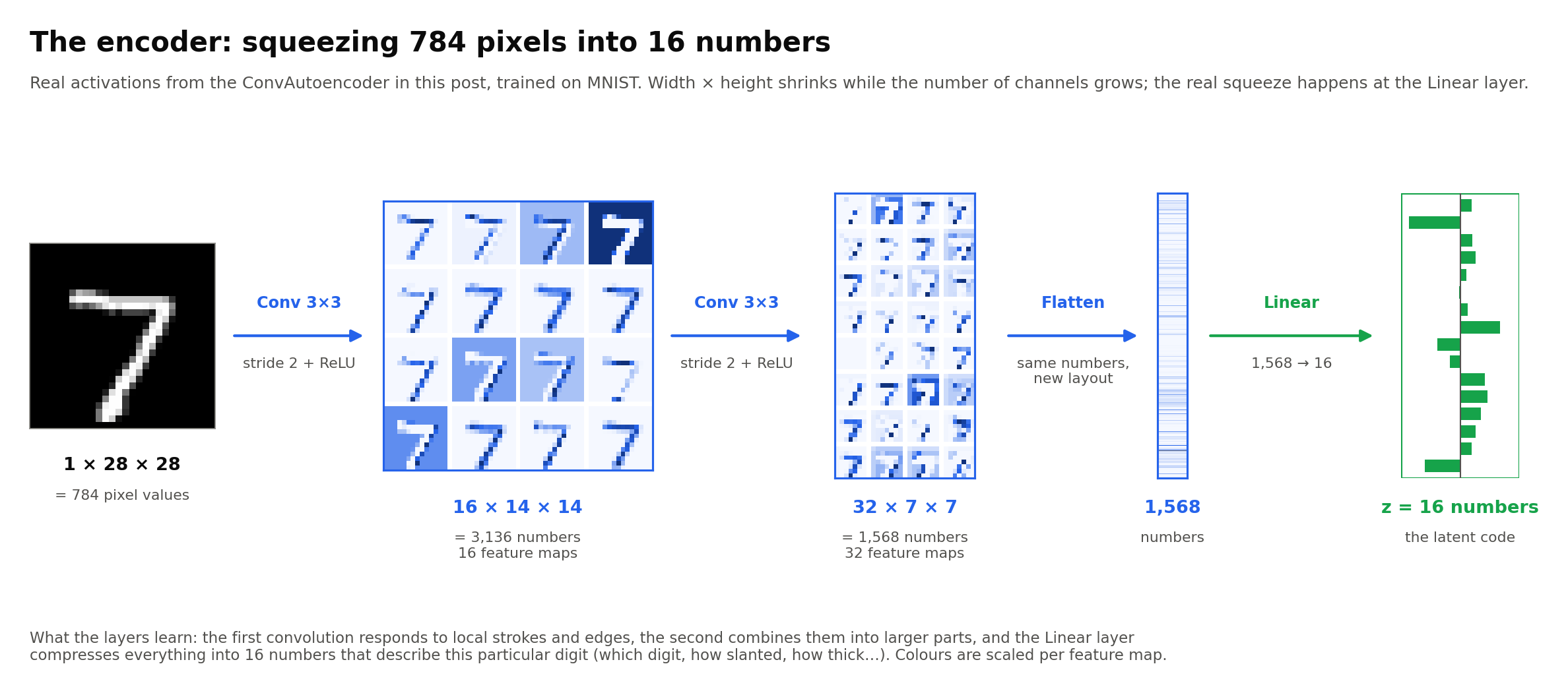
One thing worth noticing: the first convolution actually produces more numbers than the input (3,136 vs 784). Each stride-2 convolution halves the width and height, but it also adds channels, so each position is described by more features. The real squeeze happens at the very end, when a Linear layer compresses all 1,568 numbers into a latent code of only 16.
What a decoder does
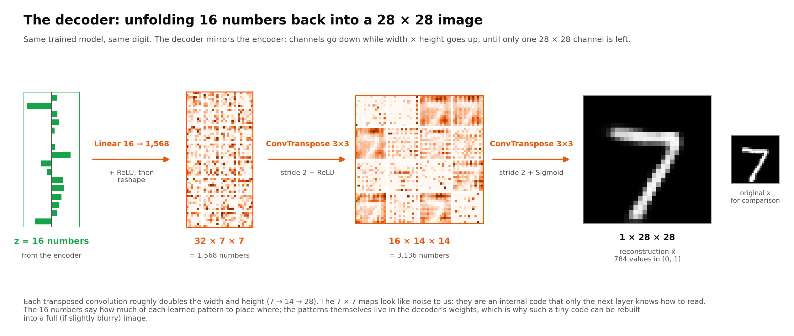
The decoder is the encoder's mirror image. It takes a low-dimensional latent code and expands it back into something with the same shape as the original input. For images, this usually means transposed convolutions (or upsampling followed by ordinary convolutions) that grow the spatial resolution step by step, while the number of channels shrinks until only the image itself is left:
Each transposed convolution works like a stamp. Every number in the smaller input grid scales a learned pattern (the kernel), and these scaled patterns are pasted into a larger output grid:
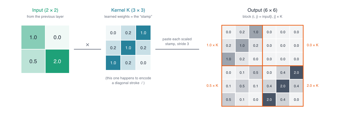
This is also why such a small code can be rebuilt into a full image. The latent code only says how much of each pattern to put where; the patterns themselves, such as what a stroke or a curve looks like, are stored in the decoder's weights.
On its own, a decoder is therefore a generator: give it a latent code and it produces an output. Whether that output makes sense, however, depends entirely on whether the code comes from a region of the latent space the decoder was trained on (more on this below).
What "auto" means
Auto comes from the Greek for "self": the network is trained to reproduce its own input. Because the target is the input itself, no labels are needed, which makes this self-supervised learning (often loosely called unsupervised learning). The architecture takes the unlabelled inputs, discovers patterns, and outputs compressed features all by itself.
The architecture
An autoencoder consists of two neural networks, the encoder and the decoder, and a bottleneck (latent space) that holds the latent codes:
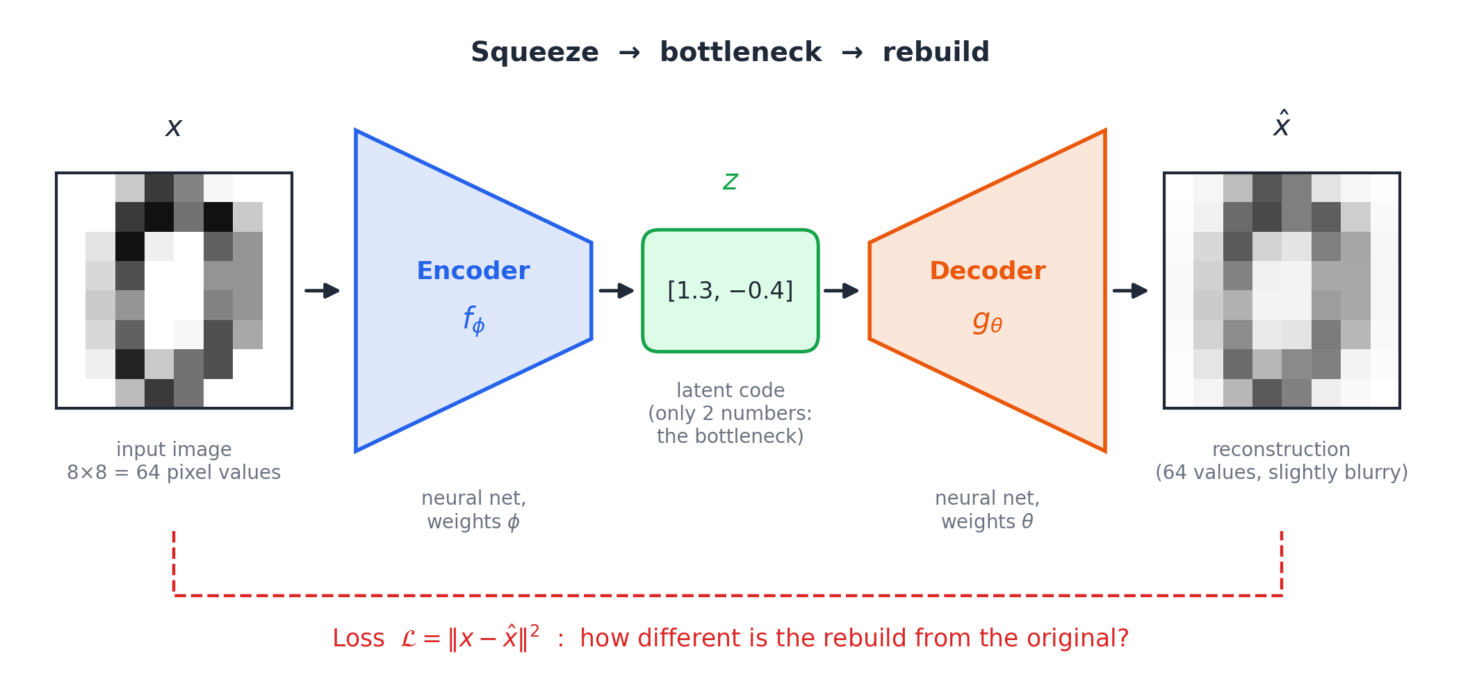
The autoencoder aims to minimise the reconstruction error, defined as:
| Symbol | Name | What it represents |
|---|---|---|
| data point | One real example, such as an image of a handwritten digit (8×8 = 64 pixel values in the diagram above; 28×28 = 784 in MNIST). | |
| encoder | A neural network with weights that maps to a latent code . | |
| latent code | The compressed representation that sits in the bottleneck, e.g. just two numbers [1.3, −0.4] in the diagram. It is a single, deterministic point: the same always gives the same . | |
| decoder | A neural network with weights that maps a latent code back to the input space. | |
| reconstruction () | The decoder's attempt to rebuild from alone. It has the same shape as , and is usually a bit blurry because some information was lost at the bottleneck. | |
| squared L2 norm | The sum of squared pixel-wise differences between and . Averaged over the pixels (and the batch), this is the familiar mean squared error (MSE). |
In practice, the loss is averaged over a training batch and minimised with gradient descent, updating and together. MSE is the default choice; when pixel values are scaled to , binary cross-entropy is also common.
What training looks like
To make this concrete, let's train a small convolutional autoencoder on MNIST, the classic dataset of 70,000 grey-scale handwritten digits, each 28×28 pixels. The encoder uses two stride-2 convolutions to go from 1×28×28 to 32×7×7, then a Linear layer squeezes that into a 16-number latent code. The decoder reverses every step with transposed convolutions. These are exactly the layers shown in the encoder and decoder figures above:
import torch
from torch import nn
from torchvision import datasets, transforms

class ConvAutoencoder(nn.Module):
    def __init__(self, latent_dim=16):
        super().__init__()
        self.encoder = nn.Sequential(                             # f_φ
            nn.Conv2d(1, 16, 3, stride=2, padding=1), nn.ReLU(),  # 1×28×28 → 16×14×14
            nn.Conv2d(16, 32, 3, stride=2, padding=1), nn.ReLU(), # → 32×7×7
            nn.Flatten(),                                         # → 1,568
            nn.Linear(32 * 7 * 7, latent_dim),                    # → z (16)
        )
        self.decoder = nn.Sequential(                             # g_θ
            nn.Linear(latent_dim, 32 * 7 * 7), nn.ReLU(),         # z → 1,568
            nn.Unflatten(1, (32, 7, 7)),                          # → 32×7×7
            nn.ConvTranspose2d(32, 16, 3, stride=2, padding=1, output_padding=1), nn.ReLU(),  # → 16×14×14
            nn.ConvTranspose2d(16, 1, 3, stride=2, padding=1, output_padding=1), nn.Sigmoid(), # → 1×28×28
        )

    def forward(self, x):
        z = self.encoder(x)
        return self.decoder(z), z

train_loader = torch.utils.data.DataLoader(
    datasets.MNIST("data", train=True, download=True, transform=transforms.ToTensor()),
    batch_size=128, shuffle=True,
)
model = ConvAutoencoder()
optimiser = torch.optim.Adam(model.parameters(), lr=1e-3)

for epoch in range(10):
    for x, _ in train_loader:          # labels are ignored: that's the "auto"
        x_hat, _ = model(x)
        loss = nn.functional.mse_loss(x_hat, x)

        optimiser.zero_grad()
        loss.backward()
        optimiser.step()
Note that the target passed to the loss is x itself. There is no y anywhere. The final Sigmoid keeps every output pixel in , the same range as the input pixels after ToTensor().
The whole thing trains in about a minute and a half on two CPU cores. Watching the reconstructions of a few test digits (which the model never trains on) shows what minimising the loss actually does:
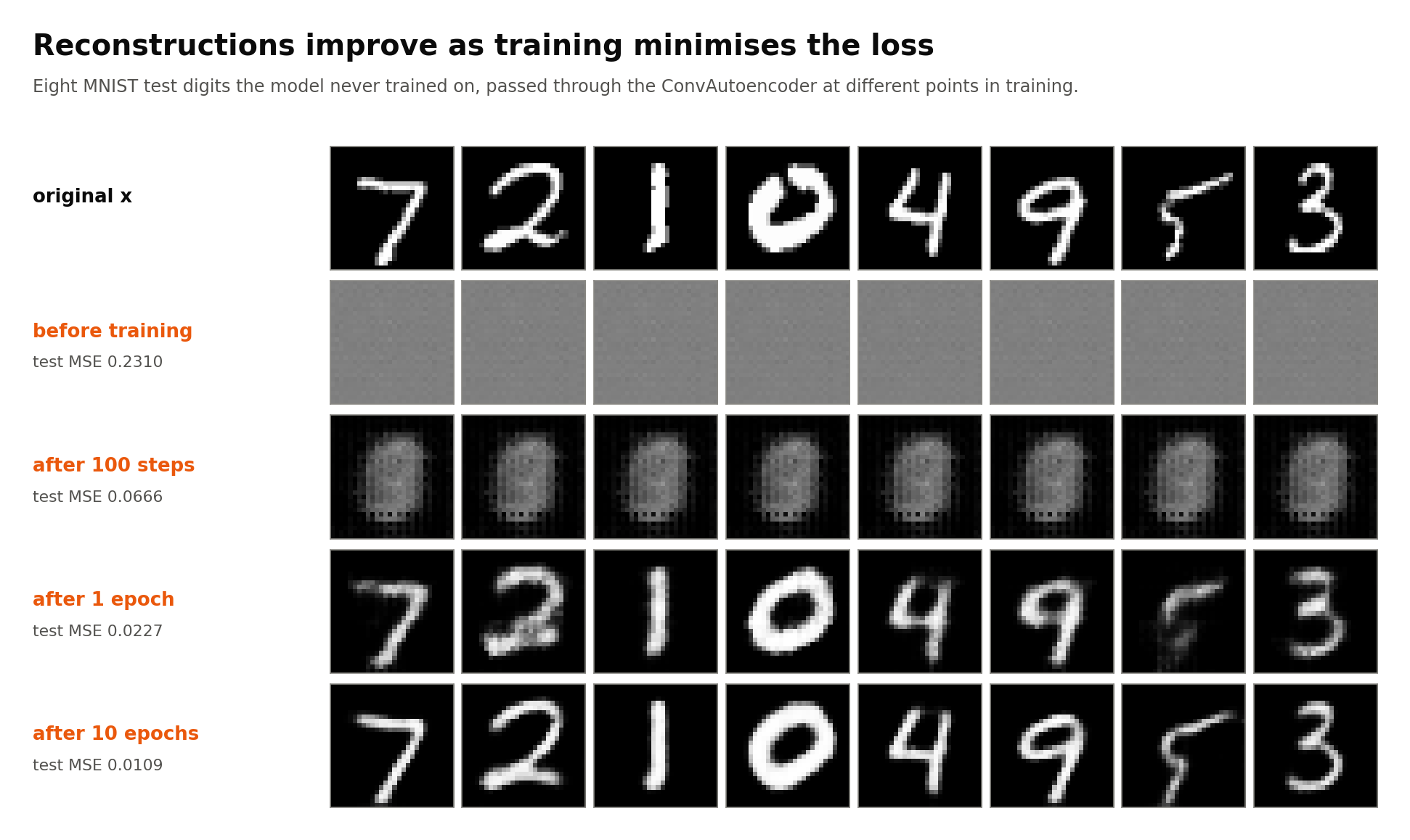
Before training, the untrained decoder outputs the same flat grey for everything. After 100 steps it has learned the cheapest trick available, which is to output a blurry "average digit" regardless of the input. By the end of the first epoch the latent code carries enough information to tell the digits apart, and after 10 epochs the reconstructions are close to the originals, just slightly softer. Notice that thin, unusual details such as the long top stroke of the 5 are the last to come through, because they matter least to the average error.
Why the bottleneck matters
Without a bottleneck, the task would be trivial. A network whose latent space is as large as the input could simply learn to copy the input to the output (the identity function) and achieve zero loss while learning nothing useful. Forcing the data through a narrow bottleneck (an undercomplete autoencoder) means the network has to decide what to keep and what to throw away, and it can only succeed by capturing the structure that most of the data shares.
The size of the bottleneck is therefore a trade-off. If it is too small, the reconstructions lose important detail and become very blurry. If it is too large, the network gets closer to memorising its inputs and the codes become less meaningful. It is also possible to use a latent space that is larger than the input (an overcomplete autoencoder), but then something else has to stop the network from simply copying, such as noise or a penalty term (see Common variants).
A useful point of reference here is PCA (principal component analysis). If the encoder and decoder are purely linear and trained with MSE, the autoencoder learns the same subspace as PCA. The non-linear activations are what let an autoencoder go beyond PCA and capture curved, more complex structure in the data.
The problem with the reconstruction error target
The loss function has only the reconstruction error term. Nothing in it says where in the latent space the codes should go or how they should be spread out. In practice, similar inputs end up with similar codes, so the encoder tends to form distinct clusters with large, empty gaps between them, and the overall scale of the space is arbitrary. This may be useful for classification tasks, but is problematic for generation tasks.
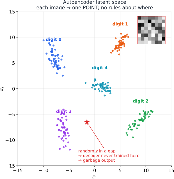
If we try to generate something new by picking a latent code that happens to land in one of those gaps, the model cannot produce a meaningful output, because the decoder was never trained on codes from that region. The same issue shows up when interpolating: walking in a straight line from the code of one digit to the code of another passes through empty space, so the intermediate outputs are often not recognisable digits.
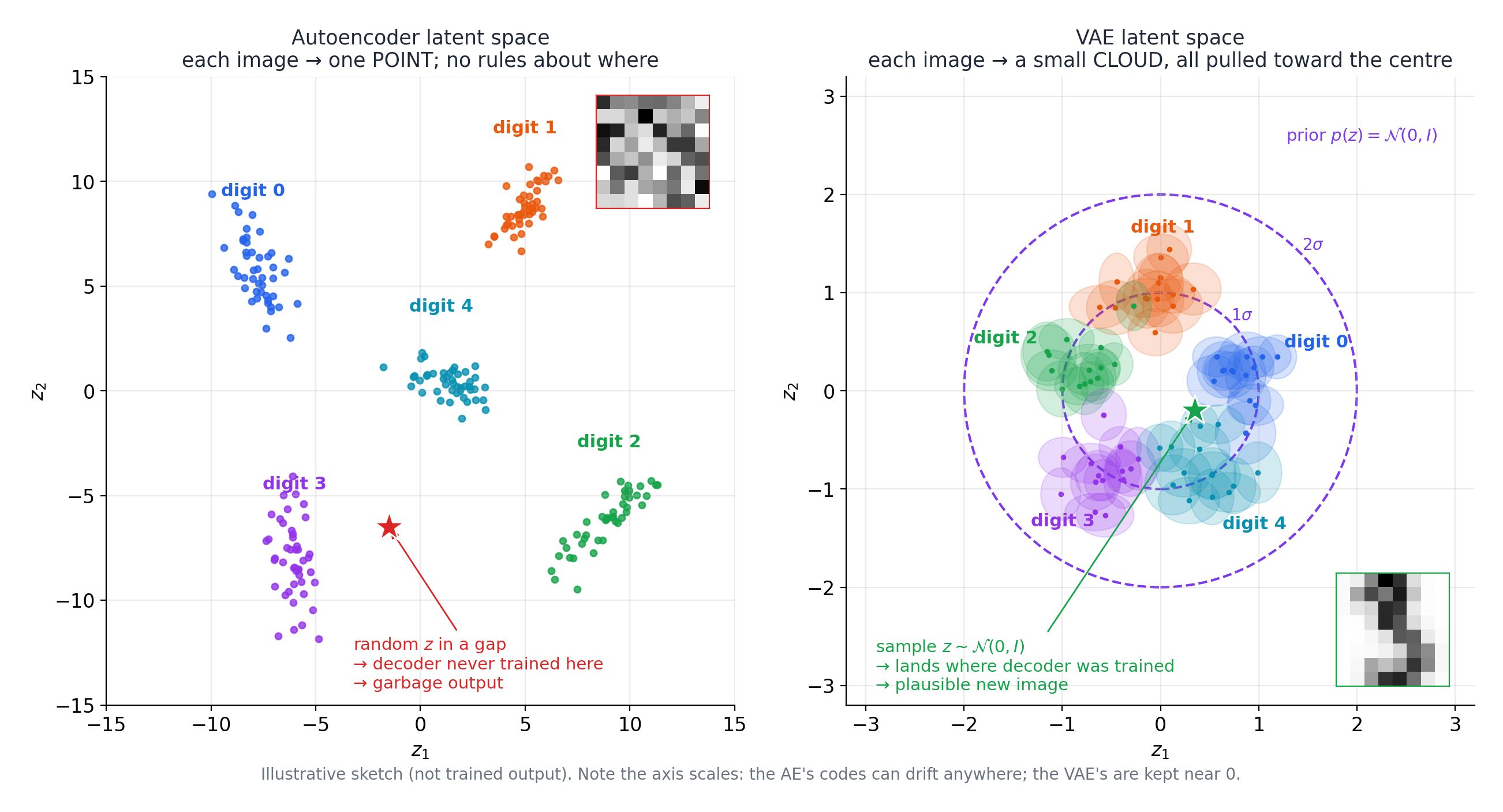
This is one of the reasons for using VAEs instead (see "Understanding VAEs (Variational Autoencoders)"), which produce probability distributions rather than single points in the latent space, and pull all of those distributions towards a shared prior (usually a standard Gaussian). This creates a smoother and more filled-in latent space with fewer gaps, leading to more consistent generations:
Common variants
The vanilla autoencoder is the starting point for a whole family of models. Most variants keep the same encoder–bottleneck–decoder shape and change either the input or the loss:
| Variant | What changes | Why |
|---|---|---|
| Undercomplete (vanilla) | Nothing; the narrow bottleneck is the only constraint. | Compression and feature extraction. |
| Denoising autoencoder (DAE) | The input is deliberately corrupted (e.g. Gaussian noise, masked pixels), but the target is the clean original. | The network has to learn what "clean" data looks like. Features become more robust. |
| Sparse autoencoder | A penalty (e.g. L1) on the latent activations is added to the loss, so only a few units are active for any given input. | Allows a large latent space without copying; tends to learn more interpretable features. |
| Contractive autoencoder | A penalty on how sensitive the code is to small changes in the input (the norm of the encoder's Jacobian). | Small perturbations of produce nearly the same , making the representation more stable. |
| Variational autoencoder (VAE) | The encoder outputs a distribution instead of a point, and a KL divergence term pulls it towards a prior. | Makes the latent space continuous and sample-able, which turns the autoencoder into a generative model. |
Use cases of autoencoders
All the examples below use the same small ConvAutoencoder from What training looks like, trained on MNIST. The only thing that changes is how we use it.
Feature discovery and dimensionality reduction
Once trained, the encoder on its own is a learned, non-linear compressor. Its latent codes can be used as compact features for downstream tasks such as clustering, search, and recommendation. With a 2- or 3-dimensional latent space, the codes can even be plotted directly to visualise high-dimensional data, as in the latent space figures above.
Similarity search is a good example. If we encode every test image into its 16-number code and then look for the codes closest to a query, we get images that look alike:
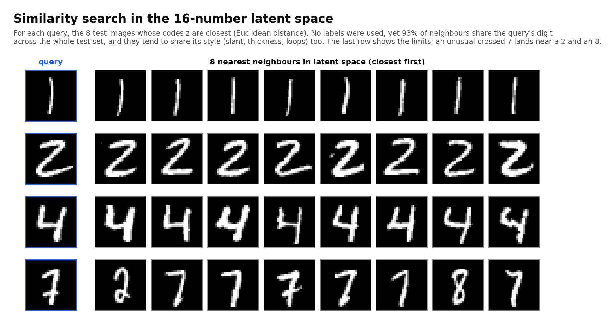
The model never saw a single label, yet 93% of the nearest neighbours share the query's digit, and they tend to share its handwriting style too. The same approach powers "find similar items" features, where comparing short codes is much cheaper than comparing raw images. The last row also shows the limits: codes capture visual similarity, not meaning, so an unusual crossed 7 ends up close to a 2 and an 8.
Keep in mind that this compression is data-specific. An autoencoder trained on handwritten digits compresses digits well but faces poorly, because it has only learned the structure of digits. Autoencoders are also a key building block in modern generative models. For example, latent diffusion models such as Stable Diffusion use an autoencoder to compress images into a much smaller latent space, and run the expensive diffusion process there instead of on raw pixels.
Denoising
A denoising autoencoder is trained on pairs of (corrupted input, clean target). The corruption is usually added artificially during training so that the clean version is always available. At inference time, it outputs a clean version of a noisy or corrupted input, e.g. removing grain from photos or cleaning up scanned documents.
To see the difference this training set-up makes, we can train the same architecture twice: once as a vanilla autoencoder (clean → clean), and once as a denoising autoencoder, where Gaussian noise was added to every input but the loss still compared the output with the clean original (noisy → clean). Here is how both handle the same noisy test digits:
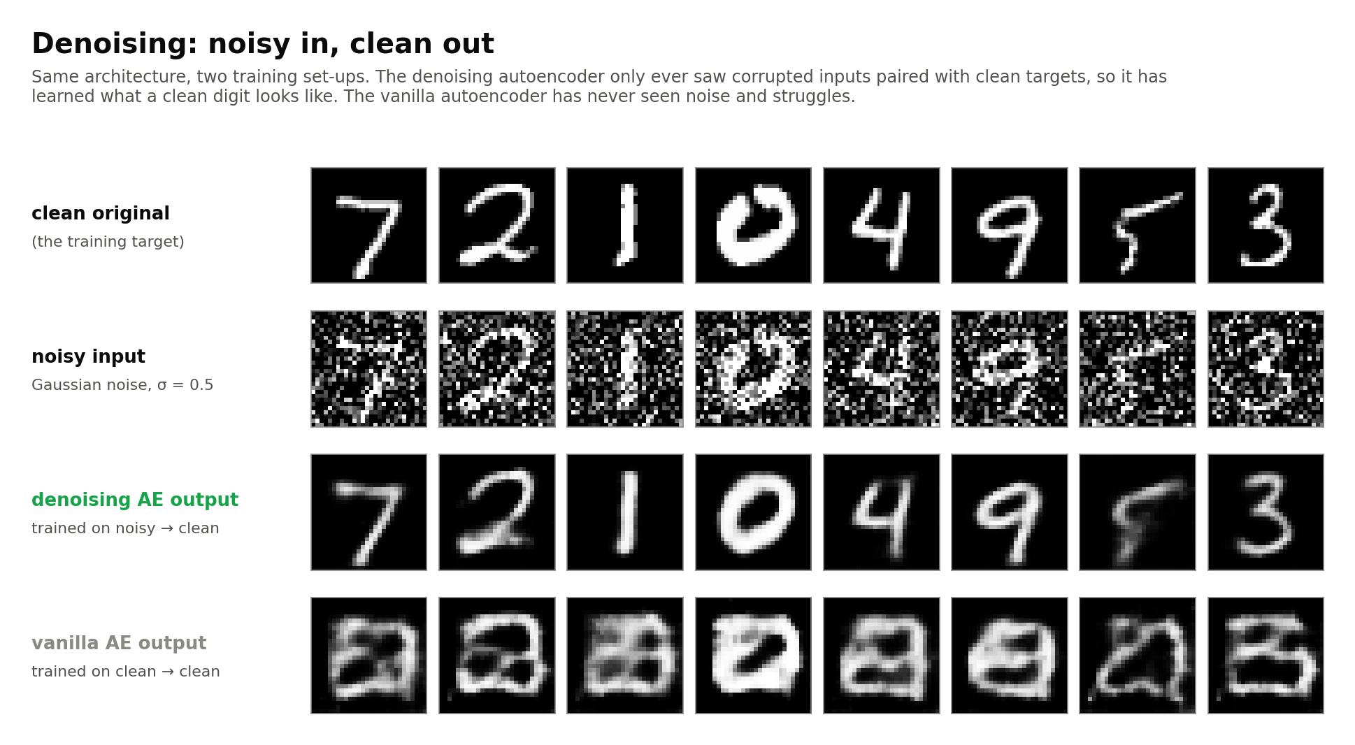
The denoising autoencoder recovers recognisable digits from inputs that are hard to read even for us, because the only way to minimise its loss was to learn what a clean digit looks like and ignore everything else. The vanilla autoencoder has never seen noise before and treats it as part of the input, so its outputs turn into blobs. The difference is entirely in the training data; the architecture is identical.
Anomaly and fraud detection
The idea is to train the autoencoder on normal data only (e.g. legitimate transactions or healthy sensor readings), so it becomes very good at reconstructing what "normal" looks like. Any input that then results in a high reconstruction error is flagged as abnormal, because the model has never learned to reconstruct that kind of pattern. The threshold is usually set from the distribution of reconstruction errors on held-out normal data, for example at the 99th percentile.
In the example below, the digit autoencoder plays the fraud detector. Handwritten digits are the "normal" data, and images of clothing from the Fashion-MNIST dataset play the role of anomalies:
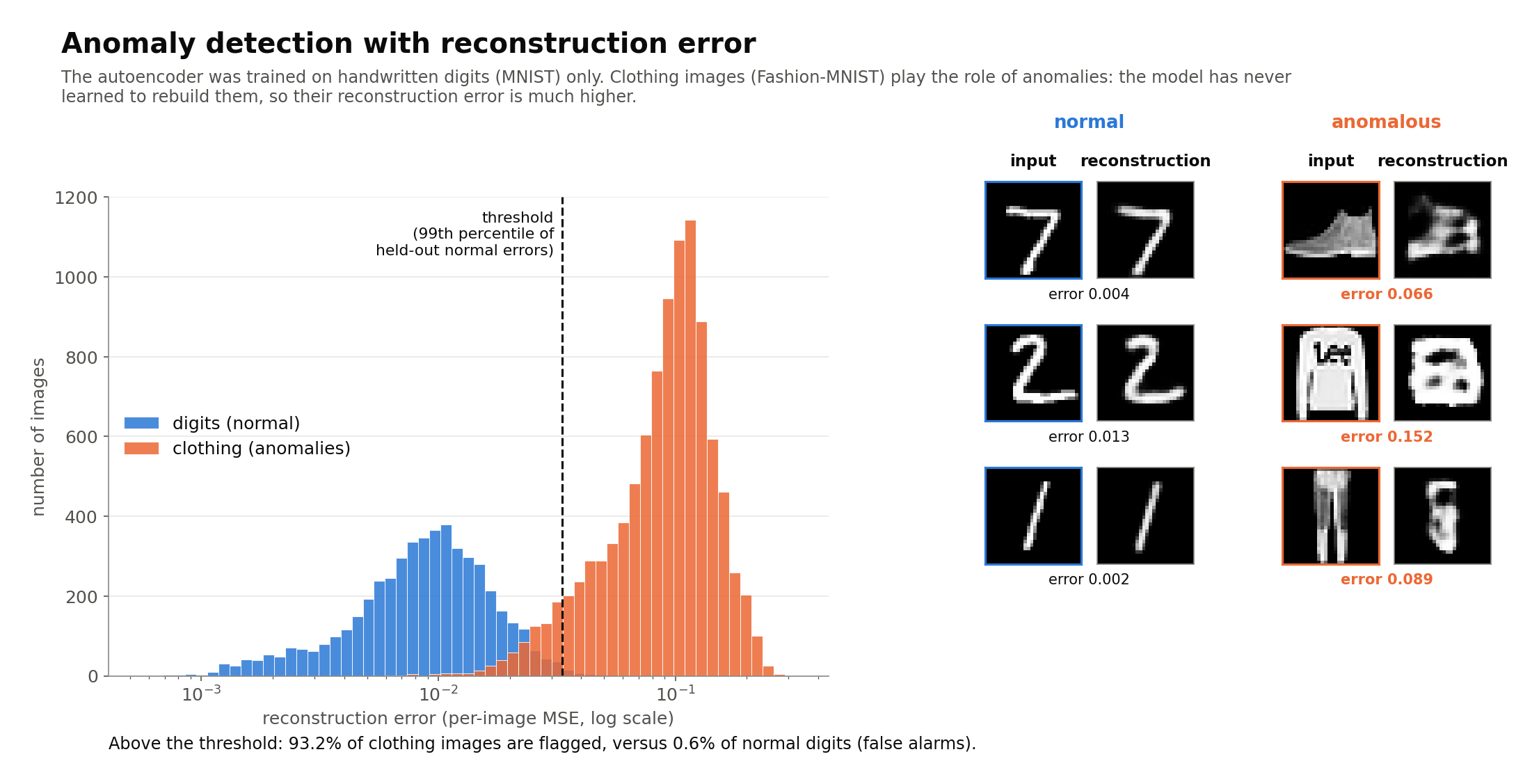
The two error distributions barely overlap. With the threshold set at the 99th percentile of errors on held-out digits, 93% of the clothing images are flagged, while only 0.6% of normal digits trigger a false alarm. The reconstructions on the right show why: when fed a shoe or a jumper, the decoder can only produce digit-like strokes, because that is all it knows how to draw.
There is a caveat, though. A sufficiently powerful autoencoder can sometimes generalise well enough to reconstruct anomalies too, which would make them look normal. The bottleneck size and the model capacity therefore need tuning, and real-world anomalies are usually much subtler than clothing among digits.
Unsupervised pre-training + classification
This use case is for when labels are expensive but unlabelled data is cheap, e.g. medical images that need an expert to label them. The process goes like this:
- First, the full encoder + decoder backbone is trained on large quantities of unlabelled data.
- Then, the decoder is removed from the network and a classifier is attached to the end of the encoder.
- A small, labelled dataset, representative of the large, unlabelled dataset, is used to train the classifier. The encoder can either be frozen (only the classifier learns) or fine-tuned along with it.
- New data -> encoder -> classifier -> class label
To test this, we can pre-train the encoder as an autoencoder on all 60,000 MNIST training images with their labels ignored, then attach a single Linear layer as the classifier and train it on only 100 to 3,000 labelled images. The baseline is the exact same network trained from scratch on the same labelled images:
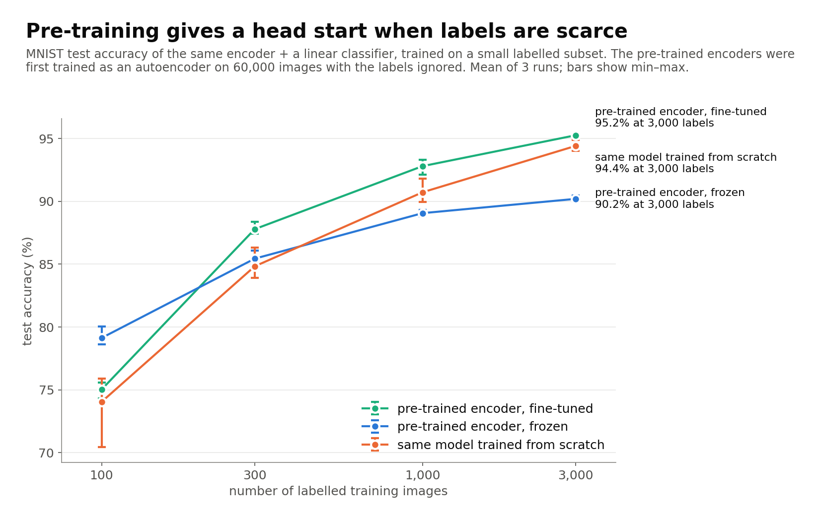
With only 100 labels, the frozen pre-trained encoder reaches 79% accuracy against 74% for the model trained from scratch, since the pre-trained features already separate the digits reasonably well. From 300 labels upwards, fine-tuning the pre-trained encoder gives the best results. The frozen encoder, on the other hand, plateaus at around 90%: features learned purely for reconstruction are not quite the features a classifier needs, and they have to be allowed to adapt. The advantage also shrinks as labels become plentiful, from about 5 points at 100 labels to under 1 point at 3,000.
This modest, shrinking gain is part of why plain autoencoder pre-training fell out of fashion once better initialisation methods and training tricks made deep networks easy to train from scratch. The idea itself lives on, though. Masked autoencoders (MAE) pre-train Vision Transformers by hiding most of an image's patches and asking the model to reconstruct them, and they are among the more effective self-supervised pre-training methods for images.
Summary
An autoencoder learns to compress its input into a small latent code (the encoder) and rebuild the input from that code (the decoder), using only the input itself as the target. The bottleneck is what forces it to learn useful structure rather than simply copying. Because the loss only rewards good reconstruction, the latent space ends up with gaps and an arbitrary layout. That is fine for similarity search, denoising, anomaly detection and pre-training, but not for generating new data. VAEs address this by encoding each input as a distribution and regularising the latent space towards a prior (see "Understanding VAEs (Variational Autoencoders)").
Resources
- Hinton, G. E. & Salakhutdinov, R. R. (2006). Reducing the Dimensionality of Data with Neural Networks. Science, 313(5786), 504–507.
- Vincent, P., Larochelle, H., Bengio, Y. & Manzagol, P.-A. (2008). Extracting and Composing Robust Features with Denoising Autoencoders. ICML.
- Rifai, S., Vincent, P., Muller, X., Glorot, X. & Bengio, Y. (2011). Contractive Auto-Encoders: Explicit Invariance During Feature Extraction. ICML.
- Kingma, D. P. & Welling, M. (2013). Auto-Encoding Variational Bayes: https://arxiv.org/abs/1312.6114
- Goodfellow, I., Bengio, Y. & Courville, A. (2016). Deep Learning, Chapter 14: Autoencoders: https://www.deeplearningbook.org/contents/autoencoders.html
- He, K. et al. (2021). Masked Autoencoders Are Scalable Vision Learners: https://arxiv.org/abs/2111.06377
- MNIST: LeCun, Y., Cortes, C. & Burges, C. J. C. The MNIST database of handwritten digits.
- Fashion-MNIST: Xiao, H., Rasul, K. & Vollgraf, R. (2017). Fashion-MNIST: a Novel Image Dataset for Benchmarking Machine Learning Algorithms: https://arxiv.org/abs/1708.07747