From Points to Clouds — How VAEs Learn to Generate

• What "variational" means in plain English
• VAE vs AE: the architectural differences
  • 1. Encoder output
  • 2. Loss function
• Sampling: where z comes from
• Use cases
• Wrapping up
• Further reading

In my post on autoencoders, I ended on a problem: an autoencoder squeezes every input into a single point in the latent space, and nothing stops those points from scattering into isolated clusters with big empty gaps between them. That is fine for compression, but if we pick a random code and ask the decoder to turn it into something new, we usually get garbage.

A variational autoencoder (VAE) fixes this with two small changes: the encoder outputs a distribution instead of a point, and the loss gets an extra term that keeps all those distributions close to a shared prior. This post walks through both changes, and then through the part that took me longest to get: how and why z is drawn differently during training, reconstruction and generation.

What "variational" means in plain English

The name comes from variational inference, a family of methods from statistics. When a quantity is too hard to compute exactly, we pick a simpler family of distributions and search within it (i.e. vary its parameters) for the member that best approximates the quantity we actually want.

In a VAE, the quantity we want is the posterior $p(z \mid x)$: given an image $x$, which latent codes $z$ could have produced it? Computing it exactly would require $p(x) = \int p(x \mid z)\,p(z)\,dz$, an integral over every possible $z$, which is intractable for a neural-network decoder. So instead, the encoder learns an approximation $q_\phi(z \mid x)$ and is restricted to a simple shape: a Gaussian with one mean and one variance per latent dimension.

In plain English, rather than answering "which exact $z$ produces this $x$?", a VAE answers "which region of $z$'s could plausibly produce something close to $x$?" Any $z$ drawn from that region should decode to something that looks like $x$.

VAE vs AE: the architectural differences

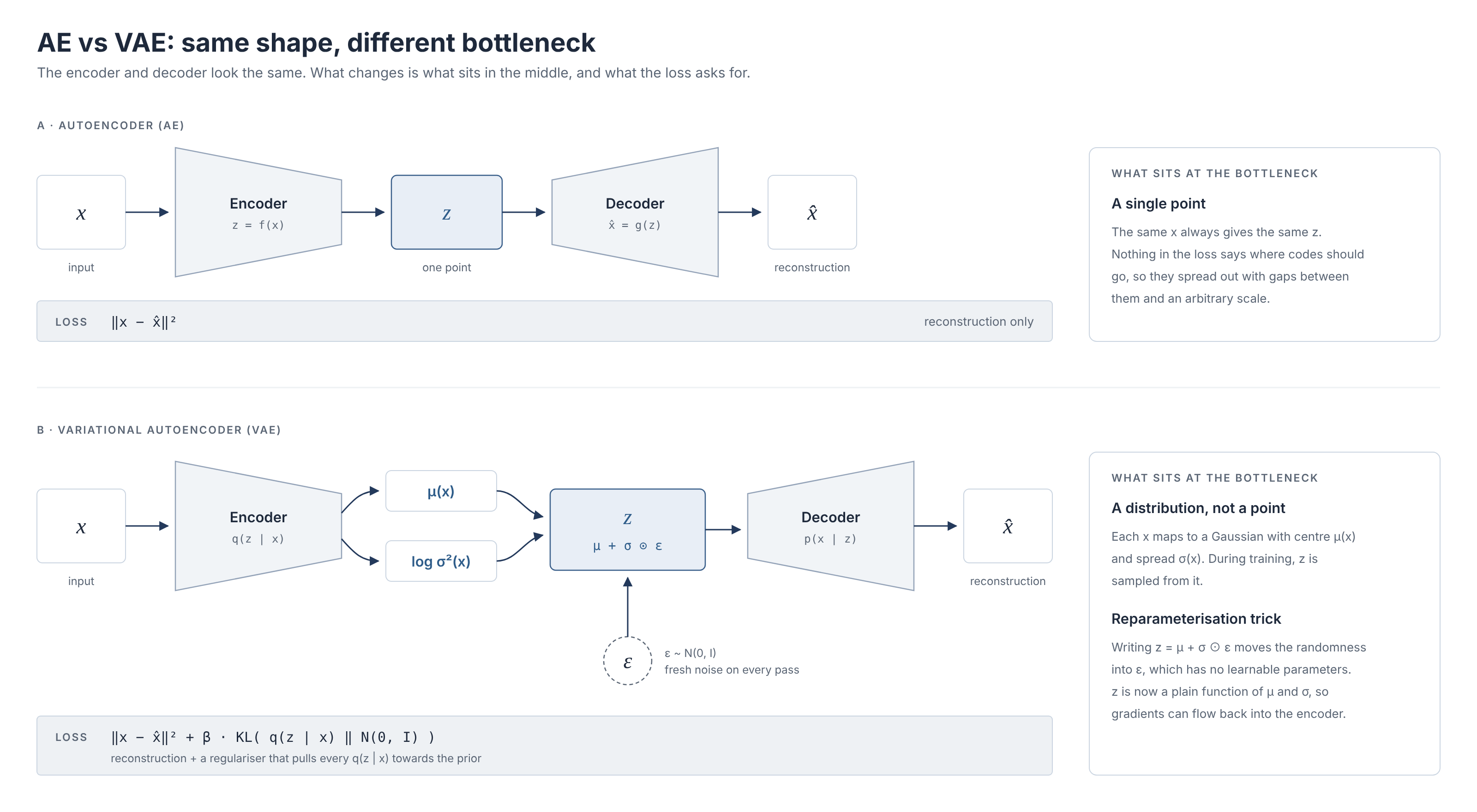
From the outside, the two networks look almost identical. The differences sit at the bottleneck and in the loss:

1. Encoder output

An AE encoder outputs a vector of z_dim numbers, which is a single, fixed point in the latent space. A VAE encoder outputs 2 * z_dim numbers per input instead: a mean $\mu$ and a log-variance $\log\sigma^2$ for each latent dimension. Together they describe a Gaussian "cloud" in the latent space rather than a point.

Here is a simplified version of the Encoder I implemented for my project training a conditional VAE on the MNIST dataset:

class Encoder(nn.Module):
    def __init__(self, z_dim):
        super().__init__()
        self.encoder_backbone = nn.Sequential(...)   # convolutions, flattening, etc.
        self.encoder_head = nn.Sequential(
            nn.Linear(256, 2 * z_dim)
        )

    def forward(self, x):
        x = self.encoder_backbone(x)
        x = self.encoder_head(x)
        mu, logvar = torch.chunk(x, 2, dim=1)
        return mu, logvar

Note that the choice of which half of the 2 * z_dim numbers become mus and which half become logvars is arbitrary. Before training, they are just numbers. They only become means and log-variances because of how we use them later (in the sampling step and in the KL term), so any consistent split works:

mu, logvar = torch.chunk(mu_logvar, 2, dim=1)
# Or
logvar, mu = torch.chunk(mu_logvar, 2, dim=1)
# Or
mu = mu_logvar[:, 0::2]
logvar = mu_logvar[:, 1::2]
# Or any other ordering, as long as there are equal numbers of mus and logvars

Why the log-variance and not the variance itself? A variance must be positive, but a Linear layer can output any real number. Predicting $\log\sigma^2$ lets the network output whatever it likes, and $\sigma = e^{0.5 \cdot \log\sigma^2}$ is always positive. It is also numerically more stable when variances get very small.

With a distribution per input, there are now two kinds of distribution worth telling apart:

1. The individual posterior $q_\phi(z \mid x)$: the small Gaussian cloud defined by the mu and logvar the encoder outputs for one image.
2. The aggregate posterior $q(z) = \frac{1}{N}\sum_{i=1}^{N} q_\phi(z \mid x_i)$: all the individual clouds averaged over the whole dataset.

We usually choose the prior to be a standard normal, $p(z) = \mathcal{N}(0, \mathbf{I})$. The KL term in the loss (next section) pulls every individual cloud towards it, while the reconstruction term pushes back: to rebuild a specific image, its cloud has to stay fairly narrow and in its own spot. The result is a compromise. Each individual cloud stays small, but together they fill the prior, so it is the aggregate that ends up close to $\mathcal{N}(0, \mathbf{I})$:

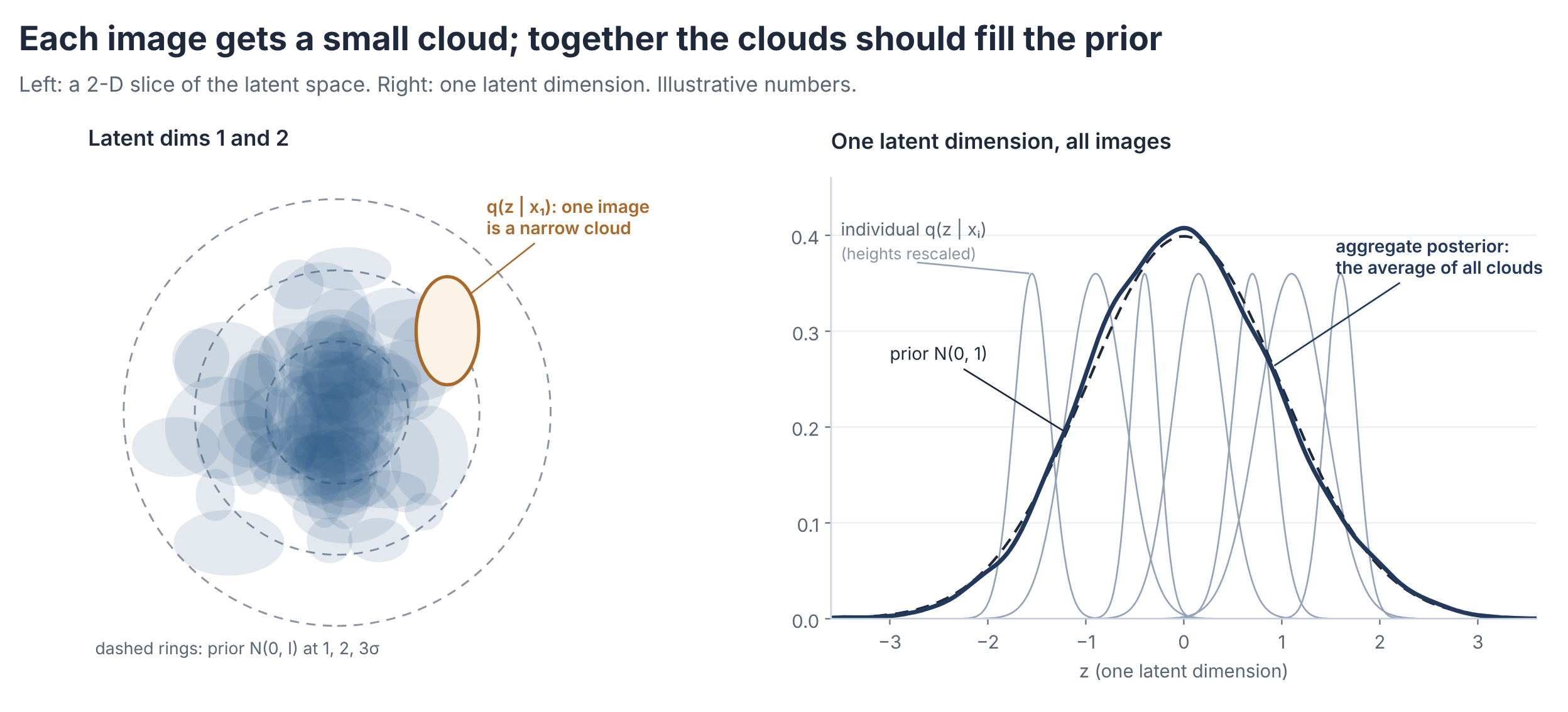
This matches what I saw when I inspected a trained model. Across test images, the $\mu$ values in each latent dimension clustered around 0 in a roughly bell-shaped spread, while the $\sigma$ values were mostly between 0.1 and 0.4: each individual cloud is narrow, yet together they cover the prior.

(If every individual cloud became $\mathcal{N}(0, \mathbf{I})$ as well, all images would map to the same cloud and $z$ would tell the decoder nothing. More on that in the $\beta$ discussion below.)

2. Loss function

Compared to an AE, the VAE loss has an additional KL divergence term:

$\mathcal{L}_{VAE} = \underbrace{\sum_{d=1}^{D} (x_d - \hat{x}_d)^2}_{\text{reconstruction}} + \underbrace{D_{\text{KL}}\big(q_\phi(z \mid x) \,\|\, p(z)\big)}_{\text{KL divergence}}$

where $D$ is the number of pixels. With a diagonal Gaussian posterior and a standard normal prior, the KL term has a closed form:

$D_{\text{KL}}\big(q_\phi(z \mid x) \,\|\, p(z)\big) = -\frac{1}{2} \sum_{j=1}^{J} \left(1 + \log \sigma_j^2 - \mu_j^2 - \sigma_j^2 \right)$

where $J$ is z_dim. Each term in the sum is smallest when $\mu_j = 0$ and $\sigma_j = 1$, so the KL term does two jobs: it pulls the clouds towards the origin (so they don't drift apart like AE codes do), and it stops them from shrinking into points (so they overlap and fill the gaps). Up to constants, the two terms together are the negative of the ELBO (evidence lower bound), the objective that variational inference maximises (I will unpack this in a separate post on the ELBO).

The two terms compete with each other. The reconstruction term wants every image to have its own sharp, well-separated code; the KL term wants every code to look like the same standard normal. The balance between them is what gives a VAE both reasonable reconstructions and a latent space we can sample from.

One practical gotcha: the reconstruction error should be summed over pixels, just as the KL term is summed over latent dimensions, and then averaged over the batch. If we use F.mse_loss with its default reduction="mean", the reconstruction error gets divided by the number of pixels (784 for MNIST), which quietly makes the KL term hundreds of times stronger than intended. For pixel values in $[0, 1]$, summed binary cross-entropy is also a common choice for the reconstruction term.

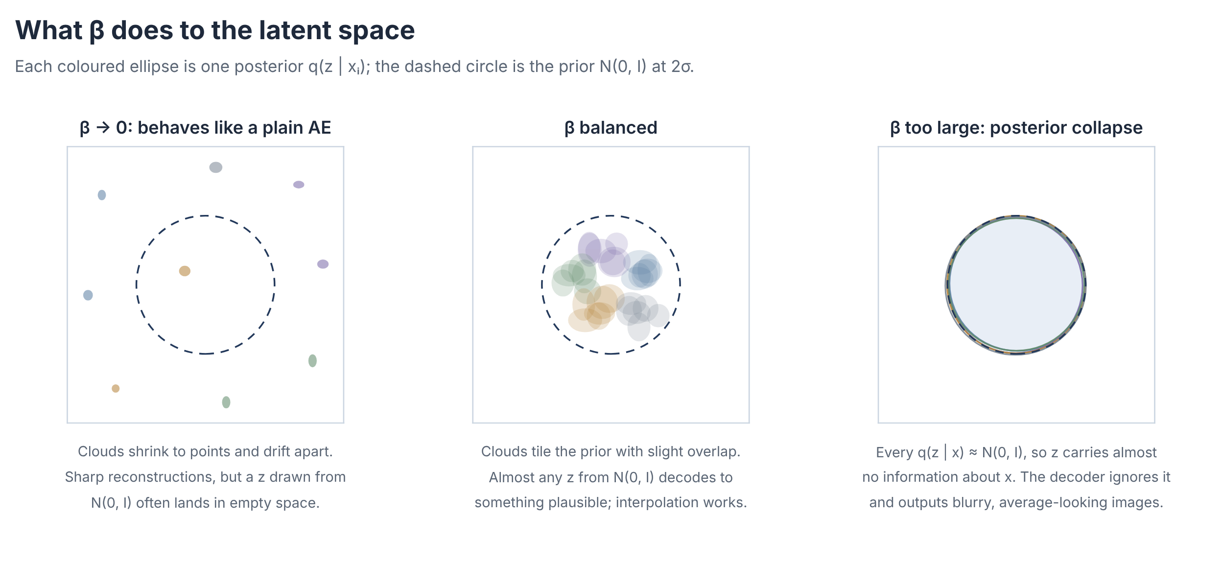
The original VAE simply adds the two terms together. A popular variant multiplies the KL term by a hyperparameter $\beta$ to control its strength:

$\mathcal{L}_{\beta\text{-}VAE} = \sum_{d=1}^{D} (x_d - \hat{x}_d)^2 + \beta \cdot D_{\text{KL}}\big(q_\phi(z \mid x) \,\|\, p(z)\big)$

• Low $\beta$: the reconstruction term dominates. The clouds shrink towards points and drift apart, and the model behaves more and more like a plain AE: sharp reconstructions, but a $z$ drawn from $\mathcal{N}(0, \mathbf{I})$ often lands in empty space and generations come out inconsistent or broken. At $\beta = 0$, nothing stops $\sigma$ from shrinking towards zero, so it is effectively an AE with a little noise.
• High $\beta$: the KL term dominates and every cloud collapses onto the prior. This is called posterior collapse: $z$ carries almost no information about the input, the decoder learns to ignore it, and both reconstructions and generations come out blurry and average-looking.
• Balanced $\beta$: the clouds tile the prior with slight overlaps. Almost any $z$ from $\mathcal{N}(0, \mathbf{I})$ decodes to a plausible image, and walking between two codes gives smooth transitions.

A common trick to avoid collapse early in training is KL annealing: start with $\beta$ near 0 and ramp it up over the first few epochs, so the encoder learns useful codes before the KL term starts squeezing them (Bowman et al., 2016).

Sampling: where z comes from

When I was studying AEs and VAEs, I realised that the key to fully understanding these architectures, and the reasoning behind their design, is to understand how the latent space is organised and how z is obtained in each case.

As touched on in my autoencoders post, the codes of an AE form clusters that can land anywhere in the latent space. In a VAE, each input maps to a Gaussian cloud instead, and all the clouds are pulled towards the prior:

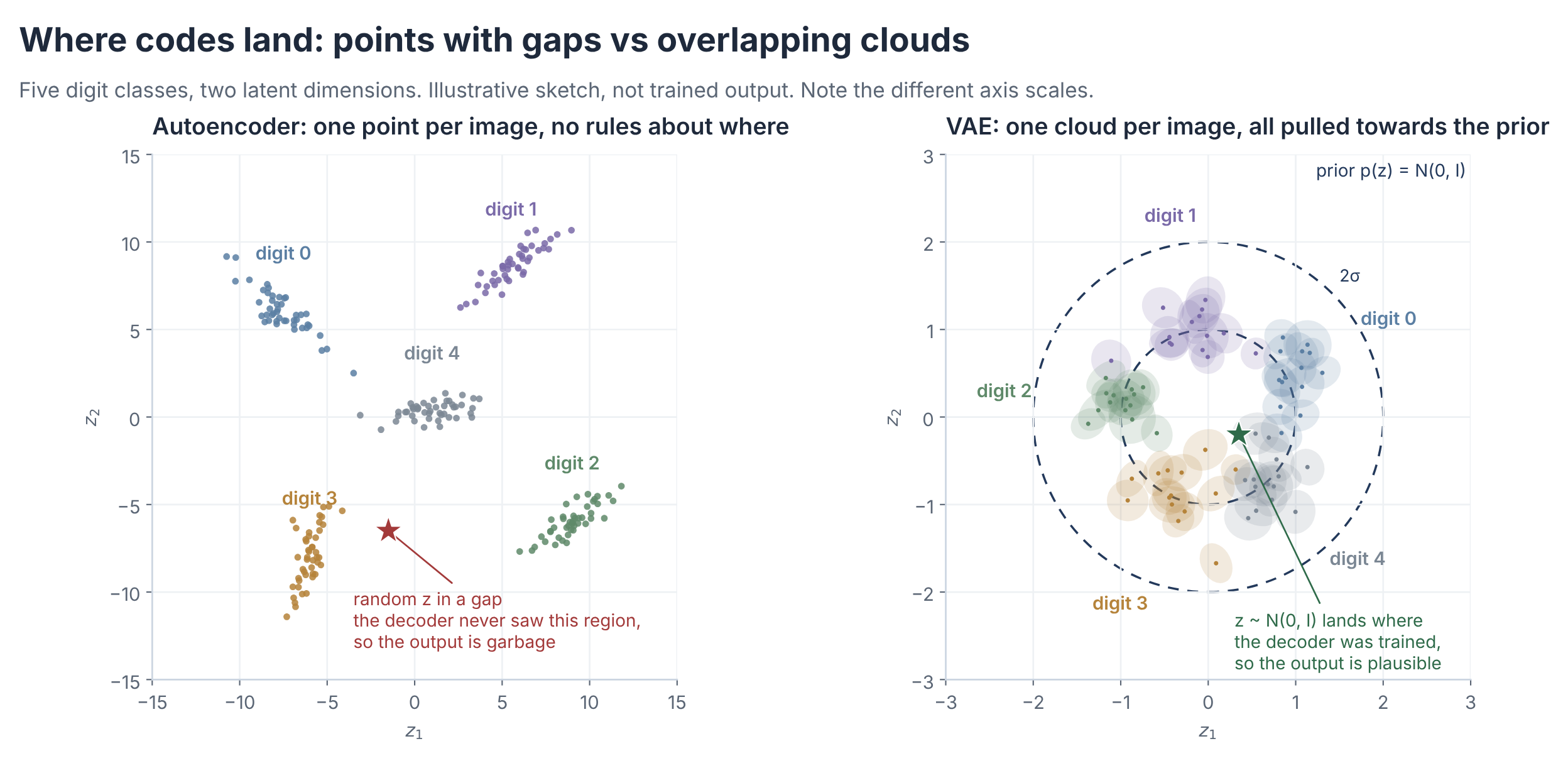
With an AE, there is no sampling at all. The encoder is deterministic, and whatever code it outputs goes straight into the decoder. If we want to generate something new, we have to pick a code ourselves and hope it doesn't land in a gap.

With a VAE, it gets more interesting, because we get z in a different way depending on what we are trying to do:

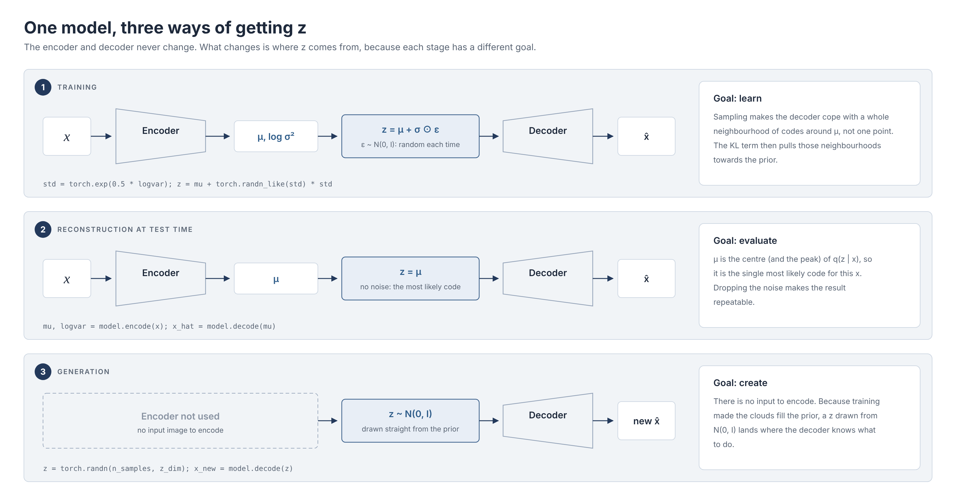
In training, our goal is to learn, so we draw a random sample from $\mathcal{N}(\mu, \sigma^2)$, using the $\mu$ and $\sigma^2$ the encoder produced for that input. There are three reasons for this:

1. It teaches the decoder a region, not a point. The same image gives a slightly different z every time it is seen, so the decoder has to map the whole neighbourhood around $\mu$ to something that looks like that image. As a result, nearby codes decode to similar images, which is exactly what makes the latent space smooth.
2. It is what makes $\sigma$ matter. If we always decoded $\mu$, the variance would only appear in the KL term, which would happily push it to 1 at no cost, and the clouds would mean nothing. With sampling, a larger $\sigma$ means noisier codes and worse reconstructions, so the reconstruction term and the KL term have to negotiate over how wide each cloud should be.
3. It is how the reconstruction term is estimated. Strictly speaking, the loss asks for the average reconstruction error over all the $z$'s in the cloud. We can't evaluate every possible $z$, so we take one random sample per training step. Any single estimate is noisy, but over thousands of steps it averages out.

Sampling on its own would break backpropagation, because a random draw has no gradient with respect to $\mu$ and $\sigma$. The reparameterisation trick gets around this by drawing the noise separately and then shifting and scaling it:

std = torch.exp(0.5 * logvar)
eps = torch.randn_like(std)   # ε ~ N(0, I), no learnable parameters
z = mu + eps * std            # z is now a differentiable function of mu and std

The randomness lives entirely in eps, so gradients can flow through mu and std back into the encoder.

In reconstruction, our goal is to evaluate, not to optimise. The $\mu$ from the encoder is both the centre and the peak of a Gaussian, so it is the single most likely code for the input image. We simply use it for decoding, which also makes the result repeatable.

In generation, our goal is neither to evaluate nor to optimise. We want to get something new out of a trained model, and there is no input image to encode. What we do know is that training pushed the aggregate posterior towards the prior $\mathcal{N}(0, \mathbf{I})$, so a $z$ drawn from the prior should land in a region the decoder knows how to handle. That is why we sample from the prior. We get something plausible, but we don't get to choose what.

Use cases

Since almost any $z$ drawn at random from an AE's latent space lands somewhere the decoder never saw during training (and higher dimensionality only makes the empty space larger), traditional AEs are poor at generation tasks.

A VAE's latent space is more organised and smoother, which makes it much better suited to:

• Generation: drawing new samples from the prior.
• Interpolation and latent arithmetic: walking from one code to another, or adding a direction such as "smiling" to a face.
• Anomaly detection: inputs that reconstruct poorly, or whose codes land far from the prior, are likely out of distribution.
• Compression for larger models: latent diffusion models such as Stable Diffusion use a VAE-style autoencoder (with a very light KL term) to compress images into a compact latent space, and the diffusion model then works in that space (Rombach et al., 2022).

One honest limitation: VAE samples tend to be blurrier than those from GANs or diffusion models, which is why hybrids such as VAE-GANs exist.

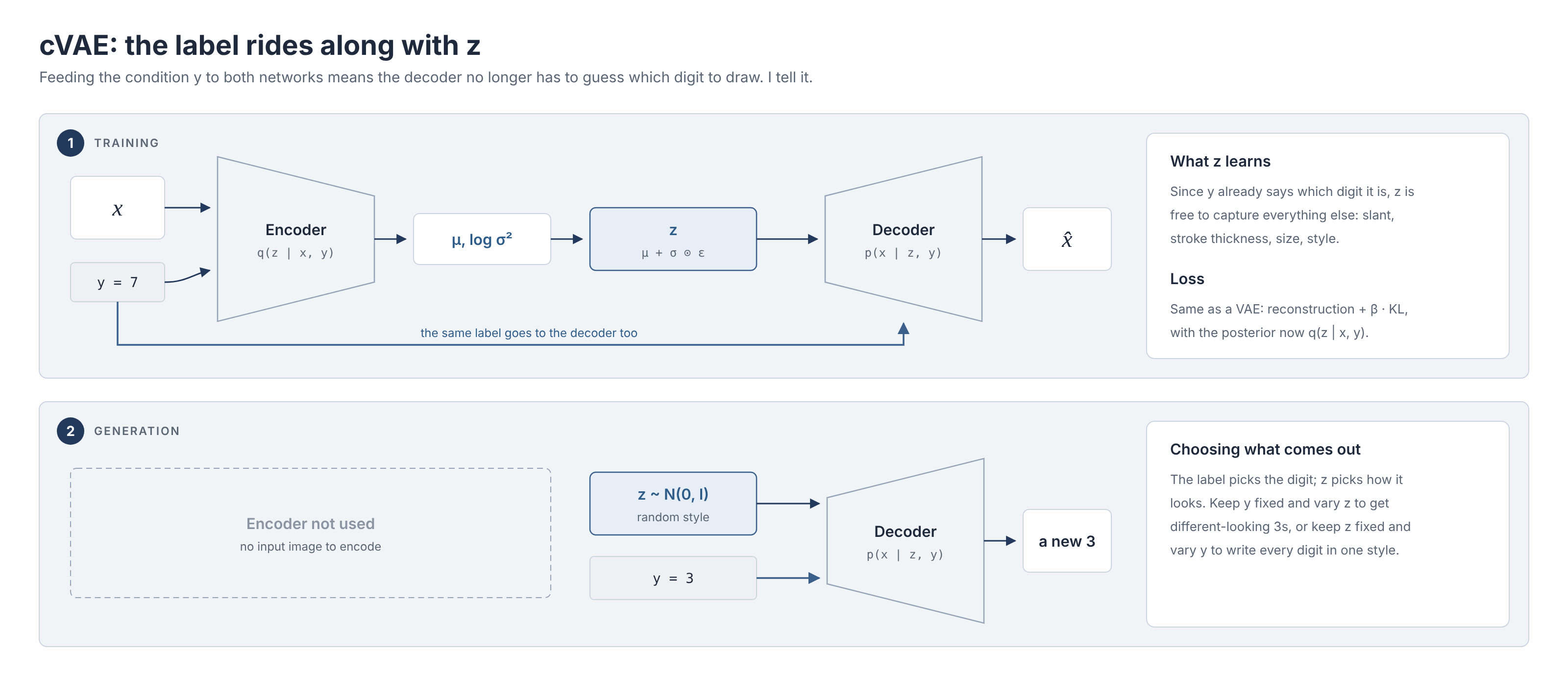
A common variation that is particularly useful for generating specific outputs is the conditional VAE (cVAE) (Sohn et al., 2015). During training, we feed the condition (e.g. the digit label) to both the encoder and the decoder. Because the label already tells the decoder which digit to draw, z is free to capture everything else: slant, stroke thickness, style. At generation time, we pass a sampled z together with the label we want, so we get something we asked for, not whatever the decoder happens to produce from a random draw:

Wrapping up

The jump from an AE to a VAE looks small on paper: two outputs instead of one at the bottleneck, plus one extra term in the loss. But it changes what the latent space is. Instead of a scatter of points with nothing in between, we get overlapping clouds that fill a known distribution, and that is what turns a compressor into a generator.

If I had to boil it down to a few points:

• The encoder outputs a distribution ($\mu$, $\log\sigma^2$) per input, not a point.
• The KL term pulls every distribution towards the prior; the reconstruction term keeps them informative. $\beta$ sets the balance.
• z is sampled in training (to learn a region), set to $\mu$ in reconstruction (to evaluate), and drawn from the prior in generation (to create).
• A cVAE adds a label to both sides, so we can choose what to generate.

I will go through the maths behind the loss in a separate post on the ELBO. Next, I want to put all of this into practice by training a cVAE on MNIST.

Further reading

• Kingma & Welling (2013), Auto-Encoding Variational Bayes: the original VAE paper.
• Kingma & Welling (2019), An Introduction to Variational Autoencoders: a longer, gentler walkthrough by the same authors.
• Doersch (2016), Tutorial on Variational Autoencoders: an intuition-first tutorial, light on prerequisites.
• Higgins et al. (2017), β-VAE: Learning Basic Visual Concepts with a Constrained Variational Framework.
• Lilian Weng, From Autoencoder to Beta-VAE: a concise overview of the whole autoencoder family.