
Training a model that scores well on a test set is only half the job. The other half starts after deployment, when the model meets data nobody tested it on and its performance quietly drifts. Debugging that drift is as important as building the model in the first place, and until this project it was something I had barely practised.
For the AI auditing project in my IFN680 unit at QUT, my teammate Clayton and I were handed three image classifiers. Each one performed almost perfectly in the studio and failed after deployment. Our job wasn't to build a better model; it was to work out why each one failed, prove it, and recommend a fix.
The three cases taught two different lessons. The first is a covariate shift: the images the model sees in the field are of a different quality from the ones it was tested on. The second and third are about spurious correlations, where a model leans on a feature that has nothing to do with what it's meant to predict, and the risks that can pose in a real product. This post covers the first case; the other two follow in later parts.
The scenario
A company built a model for a grooming app that tells bearded faces from clean-shaven ones. On its internal test set of studio photos it reached 93.7% accuracy. After launch, accuracy on photos taken in the app fell to 61.9%, and users kept reporting that it got them wrong.
The model was a ResNet-18 pretrained on ImageNet, with its final layer swapped for a two-class head. We had two test sets: 840 internal (studio) images and 740 external (mobile) images, each split evenly between the two classes. Because both sets were balanced 50/50, a change in class proportions couldn't explain the drop.
Pinning down the root cause
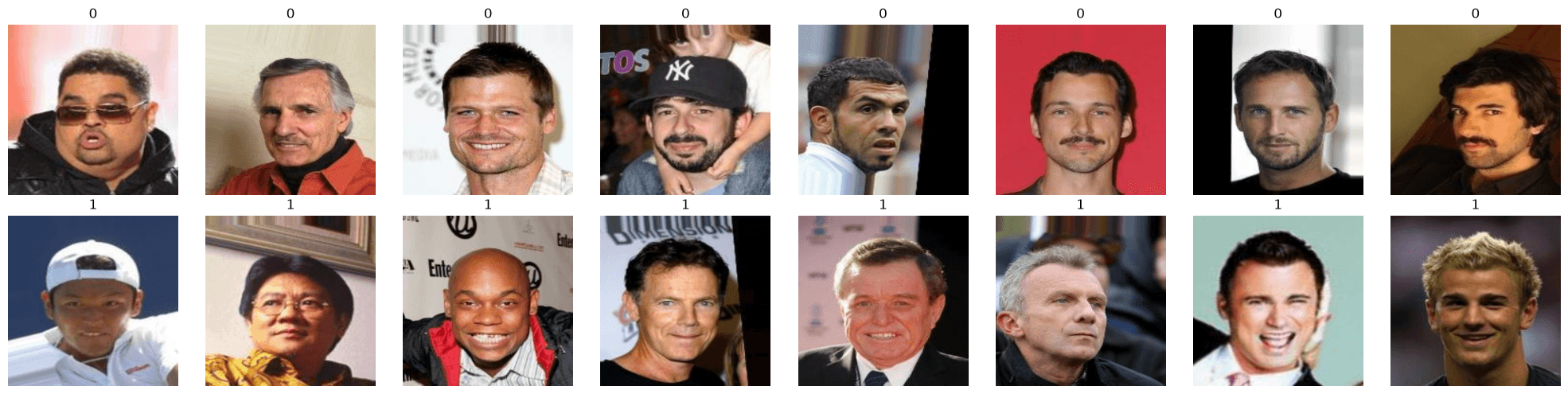
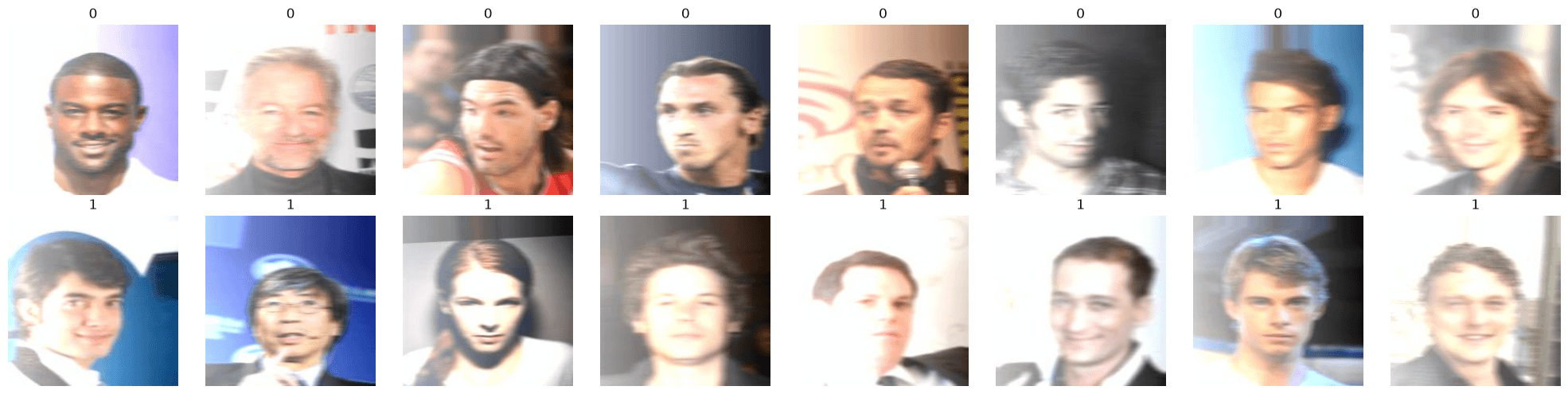
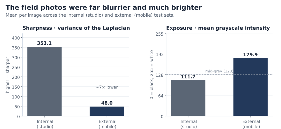
A quick visual inspection pointed straight at the likely cause. The external photos were blurry and overexposed, while the internal ones were sharp and clean, as the samples above show. The charts below tell the same story in numbers.
Seeing it was the easy part. The challenge was to measure the difference in image quality, and then to prove that it, and not something else, was what broke the model. Clayton and I ran four experiments to pin that down.
Experiment 1: measuring sharpness and exposure
We used two simple metrics.
Laplacian variance (LV) measures sharpness. The Laplacian is a filter that responds strongly to edges, so the variance of its output across an image tells you how much fine edge detail there is. Blur smooths edges away, and the score falls. It's a long-standing focus measure from autofocus research (Pech-Pacheco et al., 2000), and only a few lines of code.
Mean grayscale intensity (MGI) measures exposure. Convert the image to grayscale and average its pixel values, from 0 (black) to 255 (white).
The key findings were:
- The internal set was more than seven times sharper than the external set (mean LV 353.1 vs 48.0; the higher, the sharper).
- The external set was much brighter (mean MGI 179.9 vs 111.7).
Is there a "right" exposure value to compare against? Not a universal one, since a snowy scene should be brighter than a night shot. As a rough reference, the midpoint of the 0–255 scale is about 128, and a scene that averages out to photographic mid-grey (18% reflectance) lands at around 118 once standard sRGB gamma is applied. The studio set sits close to that; the mobile set is well over towards white. The more useful baseline, though, is the data the model was built on, and the field photos were a long way from it.
What the errors had in common
The overall accuracy hid the most telling detail: the model failed in one direction only. Here the positive class is clean-shaven, so a false positive (FP) is a bearded face classified as clean-shaven. Of the 282 errors on the external set, 278 (98.6%) were FPs. Recall for bearded faces fell from 0.91 on the internal set to 0.25 on the external set, while recall for clean-shaven faces stayed at 0.99. On blurry photos, the model almost always defaulted to "clean-shaven".
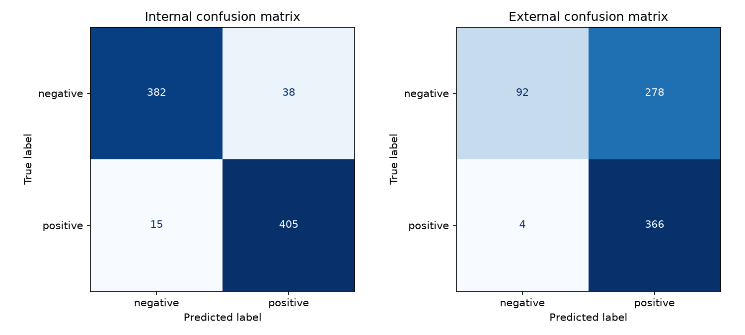
That makes sense once you think about what a beard is to a CNN: a high-frequency texture along the jaw and chin. A clean-shaven face is essentially the absence of that texture. Blur removes texture, so it can push a bearded face towards "clean-shaven" but almost never the other way round.
Three more checks pointed the same way:
- Within the external set, the misclassified bearded faces were blurrier than the ones the model got right (mean LV 50.1 vs 61.1), so blur tracked the errors even inside a single dataset.
- The ROC AUC fell from 0.985 to 0.846. The model's scores themselves had become worse at separating the two classes, so this wasn't something a different decision threshold could fix (more on reading AUC in Understanding the ROC Curve).
- Grad-CAM showed where the model was looking. On sharp faces, the heat sat squarely on the jaw and chin, exactly where a beard would be. On blurred copies of the same faces, it drifted away from the chin towards the cheek, the eyes or even the background, as if the model no longer knew where to look.
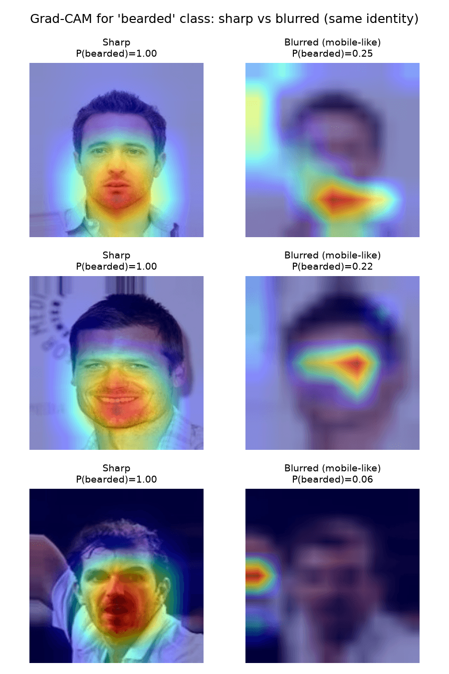
So the model had learned the right cue. Blur was destroying the signal it relied on.
Experiments 2 and 3: blurring and overexposing sharp photos
Everything so far was correlation. To show that image quality actually causes the failure, we needed to change it and nothing else.
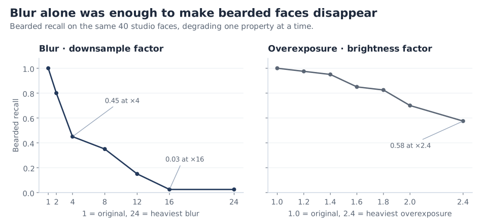
We took 40 internal bearded faces that the model already classified correctly and blurred them step by step, by shrinking each image and scaling it back up (factors from 1 to 24). Bearded recall fell steeply and steadily: 0.80 at a factor of 2, 0.45 at 4, and 0.03 by 16. We then repeated the test with brightness, from 1.0× to 2.4×. Recall dropped there too, but much more gradually, ending at 0.58.
In both experiments identity, pose and lighting stayed the same, and blur (or exposure) was the only variable that changed, so the change in recall can only come from it. Blur alone was enough to make the model miss nearly every beard; overexposure contributed, but less. This doesn't rule out every other difference between the two datasets, but it shows that image quality on its own is enough to explain the failure.
Experiment 4: retraining with blur- and exposure-augmented data
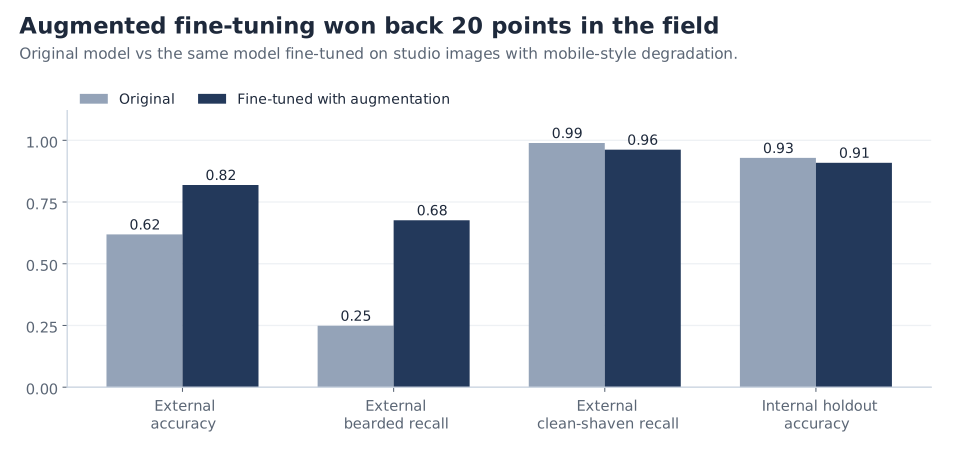
Clayton then tested a fix. He fine-tuned the whole network on 70% of the internal images, with augmentation that mimics a phone camera: random downsampling, Gaussian blur, heavy JPEG compression, and brightness and contrast jitter. External accuracy rose from 61.9% to 81.9%, and bearded recall from 0.25 to 0.68. On the other 30% of the internal images, held out from fine-tuning, accuracy barely moved (0.93 to 0.91).
One caveat: we weren't given the original training set, so the fine-tuning data came from the internal test set itself. The external set was never trained on, though, so the 81.9% is a clean number. A two-point dip on studio photos for a 20-point gain in the field is a trade I'd take.
Recommended fixes
Fix the data before fixing the model. The model was looking at the right place; it had simply never seen photos like the ones users take. Retraining on images that match the quality of the target cameras, in this case mobile phones, is the most direct fix, and experiment 4 supports it: 20 points back without touching the architecture. Real mobile photos would be best, with realistic augmentation as the next best thing.
Use a backbone that copes with degraded images. Longer term, a model pretrained on mobile photos, or one trained to be robust to blur and compression, would start from features that survive low-quality input rather than depending on fine texture.
Test on what users will actually send. A mobile-representative validation split would have caught this before launch. After launch, a sudden rise in the share of "clean-shaven" predictions is a cheap signal to monitor, because that is exactly what this failure looks like from the outside.
Wrapping up
This model wasn't broken in the usual sense. It had learned the right cue, and it would have kept working if users' photos had looked like the ones it was tested on. What changed was the data, and the only way to see that was to look past the accuracy number and start measuring the images themselves.
The next case is a different kind of failure: a model that looked just as accurate, but had learned the wrong cue altogether.