CNN Fundamentals: Kernels, Convolution, and Feature Maps

• Kernels and Filters
• How Convolution Works
• A Worked Example
• Feature Maps
• CNNs Through the Lens of NLP
  • Some Distinctions
• Resources

Convolutional neural networks are the standard architecture for finding spatial patterns in images, but the vocabulary around them, such as kernels, filters, channels, and feature maps, gets thrown around fairly loosely. This post works through what each term precisely means and how a convolutional layer actually turns an input image into an output, with a fully hand-checked numeric example. Receptive Fields in CNNs: Why Depth Beats Big Kernels of this series builds on the ideas here to explain receptive fields — why stacking small filters lets a CNN "see" a large area of the image without ever using a large kernel.

Kernels and Filters

These two words are often used interchangeably, but they describe different things:

• A kernel is a single 2D grid of learned weights, with shape H×W and exactly one channel.
• A filter is the full set of kernels applied at one layer (one kernel per input channel). A filter applied to a 3-channel (RGB) input therefore consists of three kernels, one per channel.

A filter is a single learned pattern detector: its job is to find where a specific pattern occurs in the image. A real input image contains many different patterns worth detecting (edges at various angles, colour gradients, textures), so a convolutional layer applies many filters in parallel, each specialising in a different pattern.

How Convolution Works

A filter slides across the spatial dimensions of the input, and at each position it produces exactly one output value, regardless of how many input channels it's reading from. The diagram below shows this for a 3-channel, 6×6 input with a 3×3×3 filter (one 3×3 kernel per channel), which produces a single-channel, 4×4 output:

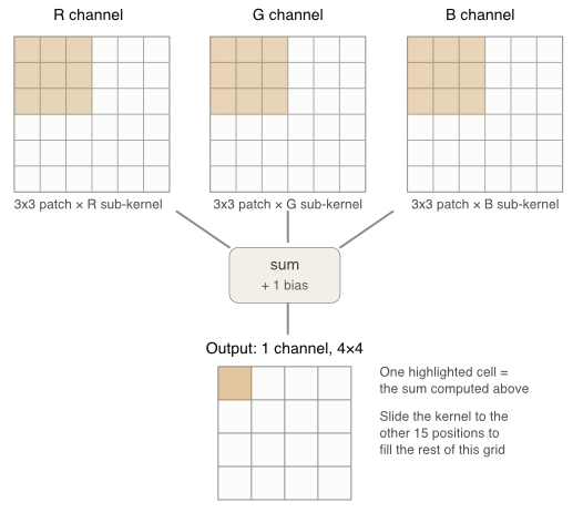
A few things worth being explicit about, since the diagram separates the channels visually but the maths doesn't:

• Convolution multiplies each channel's k×k patch by that channel's own sub-kernel, elementwise, and sums all of the resulting products together across all channels, not just within one. For a 3×3×3 filter, that's 27 products summed into a single scalar.
• A bias is added to that scalar after summing.
• One filter has exactly one bias, so the same bias value is added to every cell of that filter's output — in the diagram, the same bias is reused at all 16 positions of the 4×4 output.
• The number of input channels is fixed by what you're feeding the layer (3 for RGB, 1 for grayscale, or however many channels the previous layer output). The number of output channels is a hyperparameter: it's just how many filters you choose to apply, since each filter produces exactly one output channel.

A Worked Example

The diagram above is useful for the mechanics, but it's easier to verify correctness on a smaller example you can check by hand. Take a 3×3×3 input and a single 3×2×2 filter (one 2×2 kernel per channel):

$\mathbf{input (channel\;R)}=\begin{bmatrix} 0.1 & 0 & 0.2 \\ -0.2 & 0.3 & 0 \\ -0.1 & 0.5 & 0.1 \end{bmatrix}$

$\mathbf{input (channel\;G)}=\begin{bmatrix} -0.1 & 0.1 & 0.2 \\ 0 & 0.1 & 0.2 \\ 0 & 0 & 0.1 \end{bmatrix}$

$\mathbf{input (channel\;B)}=\begin{bmatrix} 0 & 0 & 0.2 \\ 0 & 0.1 & 0 \\ 0.1 & -0.1 & 0.2 \end{bmatrix}$

$\mathbf{kernel (channel\;R)}=\begin{bmatrix} 0.5 & 0.2 \\ 0 & 0.1 \end{bmatrix}$

$\mathbf{kernel (channel\;G)}=\begin{bmatrix} 0.1 & 0 \\ 0 & 0.2 \end{bmatrix}$

$\mathbf{kernel (channel\;B)}=\begin{bmatrix} 0 & -0.2 \\ 0 & -0.1 \end{bmatrix}$

A 2×2 kernel sliding over a 3×3 input has four valid positions, so the output (before bias) is a 2×2 grid. Working through each position — multiplying each channel's 2×2 patch by its sub-kernel elementwise and summing across all three channels:

• sum_top_left = $\begin{bmatrix} 0.1 & 0 \\ -0.2 & 0.3 \end{bmatrix}\odot\begin{bmatrix} 0.5 & 0.2 \\ 0 & 0.1 \end{bmatrix}$ + $\begin{bmatrix} -0.1 & 0.1 \\ 0 & 0.1 \end{bmatrix}\odot\begin{bmatrix} 0.1 & 0 \\ 0 & 0.2 \end{bmatrix}$ + $\begin{bmatrix} 0 & 0 \\ 0 & 0.1 \end{bmatrix}\odot\begin{bmatrix} 0 & -0.2 \\ 0 & -0.1 \end{bmatrix}$ = 0.08
• sum_top_right = $\begin{bmatrix} 0 & 0.2 \\ 0.3 & 0 \end{bmatrix}\odot\begin{bmatrix} 0.5 & 0.2 \\ 0 & 0.1 \end{bmatrix}$ + $\begin{bmatrix} 0.1 & 0.2 \\ 0.1 & 0.2 \end{bmatrix}\odot\begin{bmatrix} 0.1 & 0 \\ 0 & 0.2 \end{bmatrix}$ + $\begin{bmatrix} 0 & 0.2 \\ 0.1 & 0 \end{bmatrix}\odot\begin{bmatrix} 0 & -0.2 \\ 0 & -0.1 \end{bmatrix}$ = 0.05
• sum_bottom_left = $\begin{bmatrix} -0.2 & 0.3 \\ -0.1 & 0.5 \end{bmatrix}\odot\begin{bmatrix} 0.5 & 0.2 \\ 0 & 0.1 \end{bmatrix}$ + $\begin{bmatrix} 0 & 0.1 \\ 0 & 0 \end{bmatrix}\odot\begin{bmatrix} 0.1 & 0 \\ 0 & 0.2 \end{bmatrix}$ + $\begin{bmatrix} 0 & 0.1 \\ 0.1 & -0.1 \end{bmatrix}\odot\begin{bmatrix} 0 & -0.2 \\ 0 & -0.1 \end{bmatrix}$ = 0
• sum_bottom_right = $\begin{bmatrix} 0.3 & 0 \\ 0.5 & 0.1 \end{bmatrix}\odot\begin{bmatrix} 0.5 & 0.2 \\ 0 & 0.1 \end{bmatrix}$ + $\begin{bmatrix} 0.1 & 0.2 \\ 0 & 0.1 \end{bmatrix}\odot\begin{bmatrix} 0.1 & 0 \\ 0 & 0.2 \end{bmatrix}$ + $\begin{bmatrix} 0.1 & 0 \\ -0.1 & 0.2 \end{bmatrix}\odot\begin{bmatrix} 0 & -0.2 \\ 0 & -0.1 \end{bmatrix}$ = 0.17

($\odot$ denotes elementwise multiply-and-sum across the 2×2 patch) So:

$\mathbf{sum}=\begin{bmatrix} 0.08 & 0.05 \\ 0 & 0.17 \end{bmatrix}$, and the final output — after adding this filter's single bias to every cell — is $\begin{bmatrix} 0.08+bias & 0.05+bias \\ 0+bias & 0.17+bias \end{bmatrix}$.

Feature Maps

The output of one filter, once it has slid across every valid position of the input, is a feature map, i.e. the 2×2 grid of values from the example above, or the 4×4 grid in the diagram. Each cell records how strongly that filter's pattern matched at that location, so a feature map is essentially a spatial map of "where does this pattern appear in the image."

A few points worth being precise about:

• A layer with N filters produces N feature maps, which are stacked together to form the N-channel input to the next layer. This is why the output channel count of a layer always equals its number of filters.
• Strictly, the feature map is the raw output of convolution plus bias, before any nonlinearity is applied. Once a nonlinearity like ReLU is applied elementwise, the result is sometimes called the activation map. In practice the two terms are frequently used interchangeably in papers and tooling, but the distinction is: feature map = conv(input) + bias, activation map = activation(feature map).
• Early layers' feature maps tend to respond to simple, generic patterns (edges, colour blobs, corners). Because each layer's filters operate on the previous layer's feature maps rather than the raw pixels, deeper layers' feature maps respond to increasingly complex, composite patterns (textures, parts of objects, whole objects). The same feature maps that are strong evidence for "this looks like an eye" in one region can combine with others to become evidence for "this looks like a face."

CNNs Through the Lens of NLP

Language models represent words using embeddings — usually a multi-dimensional vector where each dimension captures some aspect of the word's meaning. Images have an analogous problem: a single pixel intensity rarely tells you anything meaningful on its own, so you need multiple values to describe the patterns present at a location (edges, colours, textures, and so on). CNNs solve this the same way: at every spatial location, the stack of values across all of a layer's channels forms a vector, with each channel describing one learned pattern. Stacking more filters and more layers lets that vector describe increasingly complex combinations of patterns.

Some Distinctions

The analogy is useful, but it breaks down in one important way: word embeddings start from a fixed lookup table, while CNN feature vectors are computed, not looked up.

A word embedding table is a giant matrix with one fixed row per vocabulary entry — "cat" is always row 4592, "dog" is always row 891, and so on. When the model sees the token "cat", it just retrieves row 4592; there is no computation involved in producing the vector itself, only in what happens afterward.

A CNN has no equivalent table. Every feature vector at every spatial location is computed on the fly by running the filters over the input, and that computation only has access to a small local neighbourhood, i.e. its receptive field. That neighbourhood only grows as you stack more convolutional layers, each of which widens it a bit further (this growth is the subject of Receptive Fields in CNNs: Why Depth Beats Big Kernels). There's no equivalent of "pixel-pattern #4592" that the network could look up directly, and every image, and every location within it, has to be freshly interpreted through the same shared filters.

Resources

• CNN Explainer — an interactive visualisation of a full CNN, useful for building intuition about how filters and feature maps compose.
• Understanding Convolutional Neural Networks (CNN) — LearnOpenCV