
- Part 1: Query (Q), Key (K), and Value (V) for similarities
- Part 2: The different kinds of attention
- Wrapping up
- Further reading
Transformers may feel overwhelming to learn, but the underlying concept is surprisingly straightforward. The key, I've found, is understanding what attention really is, because, as the canonical paper puts it, "Attention is all you need".
That said, I found I needed a bit of maths to really grasp it. Specifically, it helps to be comfortable with vector and matrix operations: once I could multiply two matrices and keep track of their shapes, the rest fell into place.
In this post, I'll first build up attention from scratch with Query, Key, and Value, then untangle the different kinds of attention I kept bumping into: self-attention, cross-attention, and multi-head attention.
Part 1: Query (Q), Key (K), and Value (V) for similarities
At its core, attention is about similarity, whether it's between words in the same sequence or across different sequences. Query (Q), Key (K), and Value (V) are the matrices used to calculate it, and each one plays a distinct role:
- Query (Q): "what am I looking for?" One per token: the question that token is asking of the rest of the sequence.
- Key (K): "what do I offer, as a label for matching?" One per token: how that token advertises itself so others can find it.
- Value (V): "what information do I actually give you if you pick me?" One per token: the content that gets passed along once a match is made.
The way I like to picture it is a library. My query is the topic I walk in with, the keys are the labels on the spines, and the values are what's actually inside the books. I compare my topic against every label, then read the books that match best.
Where do Q, K, and V come from?
They all come from the same place: , the token embedding matrix of the whole sequence, where is the sequence length:
Each of , , and is a linear transformation of by its own learned weight matrix:
( often equals , but it doesn't have to.)
So the same tokens get projected three different ways: once as questions, once as labels, and once as content.
From similarity scores to attention
Before walking through it step by step, here's the whole pipeline at a glance:
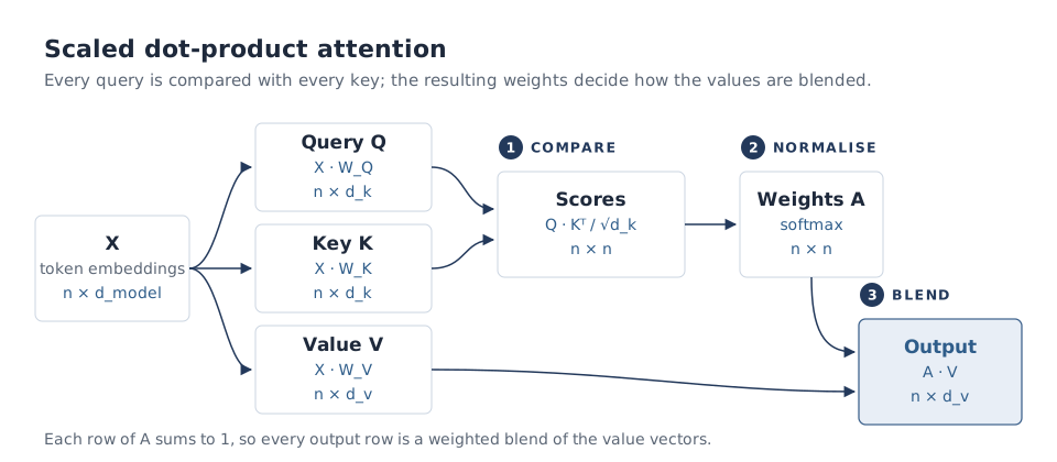
Step 1: raw scores. We compare every query against every key:
This is just dot-product similarity, and it essentially answers: given my query, which word in the sequence seems to be the best match? Row holds token 's scores against every token in the sequence (including itself).
Step 2: attention weights. We softmax each row of the scores, turning them into weights between 0 and 1 that sum to 1:
Step 3: weighted values. Finally, we multiply the weights by :
These weighted attention values are what the transformer carries forward to eventually generate tokens. Every token now has a new representation that's been "informed" by the tokens it found most relevant.
What does that look like in practice?
Take the sentence "The cat sat because it was tired." When the model processes "it", its row in might look something like this (numbers made up for illustration):
| "it" attends to → | The | cat | sat | because | it | was | tired |
|---|---|---|---|---|---|---|---|
| weight | 0.03 | 0.62 | 0.08 | 0.05 | 0.14 | 0.03 | 0.05 |
Most of the weight lands on "cat", so the new representation of "it" is mostly built out of the value of "cat". That's how the model works out what "it" refers to. What struck me is that it's a soft lookup: rather than picking one exact match, "it" gets a blend of everyone's values, weighted by how well each key matched its query.
Show me the code
The whole thing is only a few lines. Here it is in PyTorch, with the shapes tracked in the comments:
import math
import torch

torch.manual_seed(0)
n, d_model, d_k, d_v = 4, 8, 8, 8  # 4 tokens, tiny dims so we can eyeball things

X = torch.randn(n, d_model)        # [n, d_model] token embeddings

W_Q = torch.randn(d_model, d_k)    # [d_model, d_k]
W_K = torch.randn(d_model, d_k)    # [d_model, d_k]
W_V = torch.randn(d_model, d_v)    # [d_model, d_v]

Q = X @ W_Q                        # [n, d_k]
K = X @ W_K                        # [n, d_k]
V = X @ W_V                        # [n, d_v]

scores = Q @ K.T / math.sqrt(d_k)  # [n, n]   every query vs every key
A = scores.softmax(dim=-1)         # [n, n]   each row sums to 1
output = A @ V                     # [n, d_v] one blended value per token

print(A.sum(dim=-1))               # tensor([1.0000, 1.0000, 1.0000, 1.0000])
print(output.shape)                # torch.Size([4, 8])
As a sanity check, PyTorch's built-in scaled_dot_product_attention gives the same result.
Unpacking the maths, one position at a time
The matrix form is compact, but I found it much easier to see what's going on by zooming in on a single position.
- Let the current position be and another position be . The attention score of query and key is a single number (a scalar):
- After softmax across all the keys (where is the sequence length):
- The output at position is a weighted combination of the values at every position it's allowed to see. That's all positions in plain self-attention, or only the earlier ones with a causal mask (more on that below):
- Stacking the output at each position gives us the attention value matrix of the whole sequence:
- In reality, there's no computing-and-then-stacking. The whole comes out of a single matrix multiplication, , which is exactly why transformers are so GPU-friendly.
Wait, why divide by √d_k?
This little term is easy to skip over, but it matters. If the entries of and are roughly zero-mean with unit variance, their dot product is a sum of terms, so its variance grows to about and its spread to about . A quick experiment shows it:
for d_k in [4, 64, 512]:
    q, k = torch.randn(10_000, d_k), torch.randn(10_000, d_k)
    print(d_k, (q * k).sum(dim=-1).std())
# 4    ≈ 2.0
# 64   ≈ 8.0
# 512  ≈ 22.6
Big scores are bad news for softmax: it saturates, putting nearly all the weight on one token and leaving almost zero gradient for everything else.
s = torch.tensor([2.0, 1.0, 0.5])
s.softmax(-1)        # tensor([0.63, 0.23, 0.14])     nice and spread out
(s * 8).softmax(-1)  # tensor([0.9997, 0.0003, 0.0000]) basically one-hot
Dividing by brings the scores back to a sensible scale, no matter how wide the vectors are. Hence the name scaled dot-product attention.
Part 2: The different kinds of attention
The term attention gets used everywhere in transformers, and I kept running into different types of it. They can refer to very different things, despite being built on the same basic concept from Part 1, so it's worth clarifying what each one actually does.
The good news: the formula never changes. What changes is where Q, K, and V come from, and how the computation is organised.
Self-attention
- Attention weights are computed within the same sequence only.
- Q, K, and V are all projected from the same , exactly as in Part 1.
- There's no context being considered outside of the current sequence.
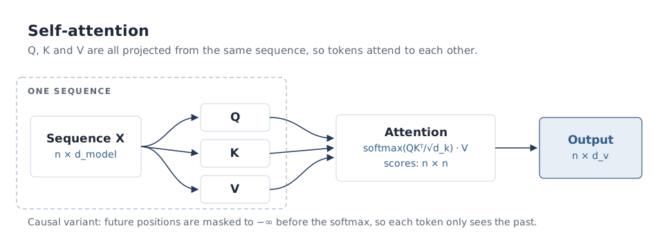
A common variant is causal (masked) self-attention, used in decoder-only models like GPT. Since the model generates text left to right, a token mustn't peek at the future. We enforce that by setting the scores above the diagonal to before the softmax, so they become 0:
           The    cat    sat    on
The       1.00     –      –      –
cat       0.30   0.70     –      –
sat       0.10   0.60   0.30     –
on        0.05   0.20   0.45   0.30
mask = torch.tril(torch.ones(n, n, dtype=torch.bool)) # lower-triangular [n, n]
scores = (Q @ K.T / math.sqrt(d_k)).masked_fill(~mask, float("-inf"))
A = scores.softmax(dim=-1) # zeros above the diagonalCross-attention
- Attention weights are computed between different sequences.
- It's most commonly used in the encoder–decoder architecture, where the decoder queries (Q) the encoder's output (K and V) for the information it needs to generate the next token.
- Think translation: while writing the French sentence, the decoder keeps "looking back" at the English one.
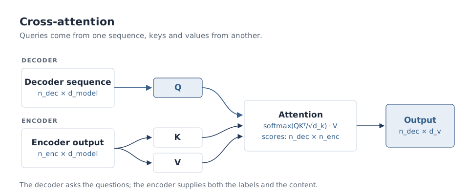
The only real change from self-attention is the input to each projection. One fun side effect: the score matrix is no longer square. It's , since every decoder token is scored against every encoder token.
def attention(Q, K, V, mask=None):
    scores = Q @ K.transpose(-2, -1) / math.sqrt(Q.size(-1))
    if mask is not None:
        scores = scores.masked_fill(~mask, float("-inf"))
    return scores.softmax(dim=-1) @ V

n_dec, n_enc = 3, 5
dec_x   = torch.randn(n_dec, d_model)  # [n_dec, d_model] what the decoder has so far
enc_out = torch.randn(n_enc, d_model)  # [n_enc, d_model] the encoder's output

Q = dec_x @ W_Q    # [n_dec, d_k]  questions come from the decoder
K = enc_out @ W_K  # [n_enc, d_k]  labels come from the encoder
V = enc_out @ W_V  # [n_enc, d_v]  content comes from the encoder

out = attention(Q, K, V)  # scores: [n_dec, n_enc] -> out: [n_dec, d_v]
Multi-head attention
This is where I got tripped up for a while. Multi-head attention is independent of both self-attention and cross-attention. It's an architecture design pattern, not a specification of attention boundaries. You can have multi-head self-attention or multi-head cross-attention.
The idea: instead of one big attention computation over the full , we split it into smaller heads, each with its own , , working in dimensions. Each head runs attention on its own, then we concatenate the results and mix them with one more linear layer, :
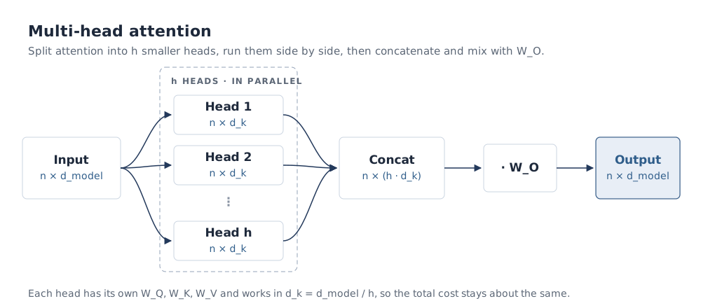
Why bother? As far as I can tell, there are three main benefits:
- Computational performance through parallelism. The heads don't depend on each other, so they're computed all at once as one batched matrix multiplication rather than one after another. And because each head works in a smaller , the total cost ends up about the same as a single full-sized head.
- More expressive power. Each head can learn to focus on a different language feature: one might track which noun a pronoun refers to, another might focus on neighbouring words. (In practice, heads don't always split the work this neatly, but the extra capacity is there.)
- Projecting back is cheap. Getting back to the expected shape is just a concatenation along the feature axis, followed by a multiplication with one linear layer () that combines the heads.
Here's a minimal version. What I like about it is how the "multiple heads" turn out to be just an extra tensor dimension:
class MultiHeadAttention(torch.nn.Module):
    def __init__(self, d_model, n_heads):
        super().__init__()
        assert d_model % n_heads == 0
        self.h, self.d_k = n_heads, d_model // n_heads
        self.W_Q = torch.nn.Linear(d_model, d_model, bias=False)
        self.W_K = torch.nn.Linear(d_model, d_model, bias=False)
        self.W_V = torch.nn.Linear(d_model, d_model, bias=False)
        self.W_O = torch.nn.Linear(d_model, d_model, bias=False)  # combines the heads

    def split(self, t):                    # [n, d_model] -> [h, n, d_k]
        n = t.size(0)
        return t.view(n, self.h, self.d_k).transpose(0, 1)

    def forward(self, x_q, x_kv, mask=None):
        Q = self.split(self.W_Q(x_q))      # [h, n_q, d_k]
        K = self.split(self.W_K(x_kv))     # [h, n_kv, d_k]
        V = self.split(self.W_V(x_kv))     # [h, n_kv, d_k]

        heads = attention(Q, K, V, mask)   # [h, n_q, d_k]  all heads in one go

        n_q = x_q.size(0)
        concat = heads.transpose(0, 1).reshape(n_q, -1)  # [n_q, h * d_k] = [n_q, d_model]
        return self.W_O(concat)            # [n_q, d_model]

mha = MultiHeadAttention(d_model=8, n_heads=2)
mha(X, X).shape            # self-attention:  torch.Size([4, 8])
mha(dec_x, enc_out).shape  # cross-attention: torch.Size([3, 8])
The same module does both self- and cross-attention. The only difference is what gets passed in as x_q and x_kv, which is the whole point: multi-head is about how attention is computed, not between what.
For a real-world implementation, I found the quantizable MultiheadAttention in PyTorch's source worth a read, since it spells out the projections and the head reshaping in plain Python.
Wrapping up
Strip away the jargon and attention is just this: compare what each token is looking for (Q) against what every token offers (K), turn those comparisons into weights, and use them to blend everyone's content (V). Everything else is a variation on where those three matrices come from and how the work is split up.
| Q comes from | K, V come from | What it's for | |
|---|---|---|---|
| Self-attention | the sequence | the same sequence | relating tokens within one sequence |
| Causal self-attention | the sequence | the same sequence, earlier tokens only | generating text left to right |
| Cross-attention | the decoder | the encoder's output | pulling in context from another sequence |
| Multi-head attention | — | — | running any of the above as parallel heads |
Once that clicked for me, the rest of the transformer started to feel a lot less overwhelming.
Further reading
- Attention Is All You Need (Vaswani et al., 2017): the paper that started it all. Section 3.2 covers everything in this post.
- The Illustrated Transformer by Jay Alammar: a very visual walkthrough of the full architecture.
- Let's build GPT: from scratch, in code, spelled out by Andrej Karpathy, which builds causal self-attention and multi-head attention line by line.